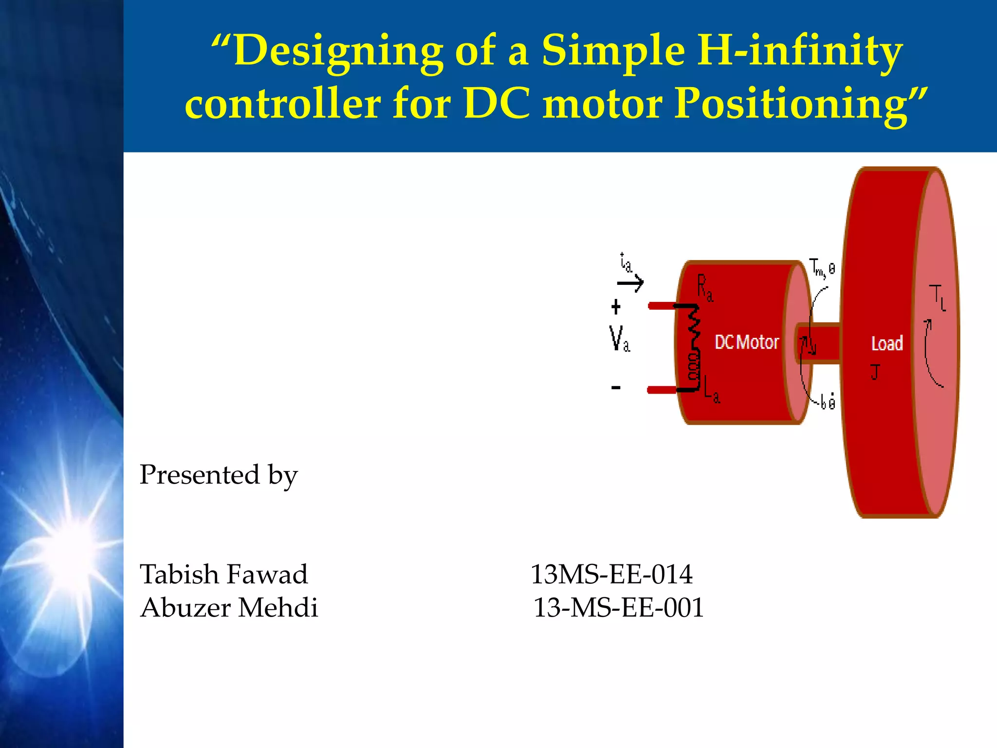
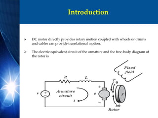
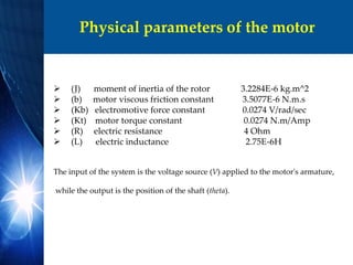
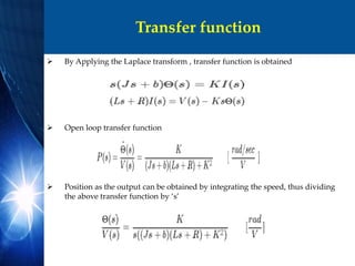
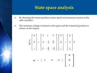
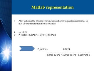
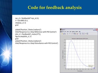
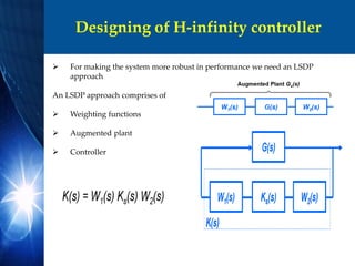
This document summarizes the design of an H-infinity controller for DC motor positioning. It describes modeling the DC motor transfer function and state space representation. PID control is designed to meet requirements of zero steady state error and settling time less than 40ms with overshoot below 16%. Simulation shows the closed loop response meets requirements. Finally, an H-infinity controller is designed using weighting functions to further improve robustness.

1. “Designing of a Simple H-infinity
controller for DC motor Positioning”
Presented by
Tabish Fawad 13MS-EE-014
Abuzer Mehdi 13-MS-EE-001

2. Contents
 Introduction
 System Equations
 Design requirements
 System modelling
 Model order reduction
 Integral control
 PID control
 Gain
 Closed loop response
 LSDP (H-infinity control)
 Conclusion

3. Introduction
 DC motor directly provides rotary motion coupled with wheels or drums
and cables can provide translational motion.
 The electric equivalent circuit of the armature and the free-body diagram of
the rotor is

4. Physical parameters of the motor
 (J) moment of inertia of the rotor 3.2284E-6 kg.m^2
 (b) motor viscous friction constant 3.5077E-6 N.m.s
 (Kb) electromotive force constant 0.0274 V/rad/sec
 (Kt) motor torque constant 0.0274 N.m/Amp
 (R) electric resistance 4 Ohm
 (L) electric inductance 2.75E-6H
The input of the system is the voltage source (V) applied to the motor's armature,
while the output is the position of the shaft (theta).

5. System Equations
 The torque generated by a DC motor is proportional to the armature current
and the strength of the magnetic field.
 The magnetic field is constant and the motor torque is proportional to the
armature current (I) by a constant factor Kt
 The back emf, e, is proportional to the angular velocity of the shaft
by a constant factor Kb.
 The torque and the back emf are constants and are equal i.e. Kt = Ke

6. Transfer function
 By Applying the Laplace transform , transfer function is obtained
 Open loop transfer function
 Position as the output can be obtained by integrating the speed, thus dividing
the above transfer function by ‘s’

7. State space analysis
 By choosing the motor position, motor speed and armature current as the
state variables.
 The armature voltage is treated as the input and the rotational position is
chosen as the output.

8. Design requirements
 We want to be able to position the motor very precisely.
 For that purpose the steady-state error of the motor position should
be zero.
 We want the steady-state error due to a constant disturbance to be
zero .
 If we simulate the reference input by a unit step input, then the
motor position output should have,
 Settling time less than 40 milliseconds
 Overshoot less than 16%
 No steady-state error, even in the presence of a step disturbance input

9. Matlab representation
 After defining the physical parameters and applying certain commands in
mat lab the transfer function is obtained.
 s = tf('s');
 P_motor = K/(s*((J*s+b)*(L*s+R)+K^2))
P_motor = 0.0274
----------------------------------------------------------
8.878e-12 s^3 + 1.291e-05 s^2 + 0.0007648 s

10. State space representation
 A = [0 1 0; 0 -b/J K/J;0 -K/L -R/L];
 B = [0 ; 0 ; 1/L];
 C = [1 0 0];
 D = [0];
 motor_ss = ss (A,B,C,D)
• motor_ss =
•
• a =
• x1 x2 x3
• x1 0 1 0
• x2 0 -1.087 8487
• x3 0 -9964 -1.455e+06
•
• b =
• u1
• x1 0
• x2 0
• x3 3.636e+05
•
• c =
• x1 x2 x3
• y1 1 0 0
•
• d =
• u1
• y1 0
Continuous-time state-space model.

11. System modelling and designing root
locus
 The main idea of root locus design is to predict the closed-loop response.
 It tells possible closed-loop pole locations and is drawn from the open-loop
transfer function.
 Then by adding zeros and/or poles via the controller, the root locus can be
modified in order to achieve a desired closed-loop response.

12. Pole Positions in root locus
 poles = pole(P_motor)
 poles = 1.0e+06 * 0 -1.4545 -0.0001
 The two open-loop poles near the origin cannot be distinguished because the
scale of the axes is set to show the third pole which is much farther to the left
than the other two poles.
 The open-loop pole located very far to the left (further than -1e6) does not
affect the closed-loop dynamics unless very large gains are used.
 We will not use gains that will make the closed-loop system unstable, we can
neglect this pole by performing a model reduction.

13. Model Order Reduction
 In general if there is a transfer function which has one (or
more) poles much farther to the left in the complex plane
(more negative) than the other poles, their effect on the
dynamic response will be hidden by the slower, more
dominant poles.
 In our case of motor position , the transient closed-loop
response for small gains will not be affected much by the
open-loop pole at -1.45e6.
 By applying this command in the mat lab the complex pole
can be avoided.
 New transfer function of the reduced order system will be
constructed to neglect the complex pole.

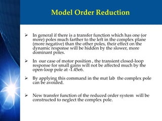
14. Model Order Reduction
 poles = pole(P_motor);
 rP_motor = minreal(P_motor*(s/max(abs(poles)) + 1))
Reduced order transfer function:
rP_motor = 2122
-------------
s^2 + 59.23 s
By checking that the other poles have not been affected by we again use the same
pole command as was used previously,
 poles(1), poles(3)] ans = 0 ans = -59.2260

15. Root locus of the reduced system
 The original root locus near the origin would closely approximate the locus
of the reduced transfer function.
 The closed-loop poles are never fast enough to meet the settling time
requirement.

16. Integral control
 Integrator is used to remove the steady-state error due to a constant
disturbance.
 This adds a 1 / s term to the forward path of the system.

17. PI control
 PI instead of I control adds a zero to the open-loop system.
 We'll place this zero at s = -20.
 C = (s + 20) / s; %Adding the zero at s=-20
 The system is stabilized zero steady-state error to a constant disturbance is
achieved.
 The system is not fast enough.

18. PID control
 Pull the root locus further to the left to make it faster.
 We placed a second open-loop zero, resulting in a PID controller.
 Two PID zeroes are at s=-60 and s=-70.
 Two of the closed-loop poles can be placed well within both the settling time
and percent overshoot requirements.
 Reduce the model again by applying the minreal command.

19. Closed loop pole location
 The one open-loop zero was cancelled, the other open-loop zero remains in the
closed-loop transfer function and cannot be neglected.
 The effect of an additional zero (if there is no cancellation) is in general to speed
up the response and add overshoot.
 We have to be conservative in picking where on the root locus we want the closed-
loop poles to lie.
 We need the settling time and the overshoot to be as small as possible, particularly
because of the effect of the extra zero.

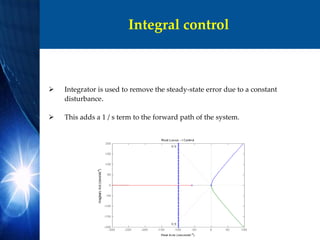
20. Determining gain
 Large damping corresponds to points on the root locus near the real axis.
 A fast response corresponds to points on the root locus far to the left of the
imaginary axis.
 To find the gain corresponding to a point on the root locus,
the rlocfind command is used.
 [k,poles] = rlocfind (rsys_ol)
 Select a point is selected on the root locus on left side of the loop, close to the
real axis.
 These pole locations indicate that the response would have almost no
overshoot if it were a canonical second-order system.
 However the presence of the zero in this system will add some overshoot.

21. Gain
selected_point = -1.3744e+002 +1.3043e+001i
k = 0.1308
poles = 1.0e+002 * -1.3874 + 0.1323i -1.3874 - 0.1323i

22. Closed loop response
 Response to a step reference the system has an overshoot of
approximately 14%.
 A settling time just under 0.04 seconds.
 No steady-state error.

23. Code for feedback analysis
sys_cl = feedback(k*rsys_ol,1);
t = 0:0.0001:0.1;
step(sys_cl, t)
grid
ylabel('Position, theta (radians)')
title('Response to a Step Reference with PID Control')
dist_cl = feedback(P_motor,k*C);
figure;step(dist_cl, t)
grid
ylabel('Position, theta (radians)')
title('Response to a Step Disturbance with PID Control')

24. Designing of H-infinity controller
 For making the system more robust in performance we need an LSDP
approach
An LSDP approach comprises of
 Weighting functions
 Augmented plant
 Controller

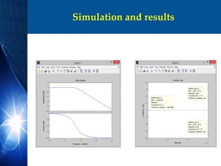
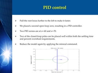
25. Simulation and results
W1=0.1*(s+100)/(100*s+1);
W2=0.1;
P=augw( P_motor,W1,W2);
GAM=0;
k = 0.1308
PM = 50.3868
• pzmap(sys_cl)
• damp(sys_cl)
• [Wn,zeta,poles] = damp(sys_cl)
• bode(sys_cl)
• zeta = -log(.16) / sqrt( pi^2 + (log(.16))^2 );
• PM = 100*zeta

26. Simulation and results

27. Conclusion
We can see that in response to a step reference the system has
 an overshoot of approximately 14%.
 a settling time just under 0.04 seconds.
 No steady-state error.
 The response to a step disturbance reaches a steady-state value of zero.
 All of the design requirements have been met.