This document discusses transfer functions and their derivation from electrical circuits and control systems. It begins by defining a transfer function as the ratio of the Laplace transform of the output variable to the Laplace transform of the input variable. Examples are then given of deriving transfer functions from simple RLC circuits by applying Kirchhoff's laws and taking the Laplace transform. The document also discusses deriving transfer functions from block diagrams of open-loop and closed-loop control systems and provides rules for reducing complex block diagrams to a single transfer function relating the input to the output.

1. E3145/6/1
THE TRANSFER FUNCTION
THE TRANSFER FUNCTION
OBJECTIVES
General Objective : To understand and interpret the concept of transfer
function.
Specific Objectives : At the end of the unit you will be able to :
 State the definition of transfer function.
 Identify the transfer function from a simple electric
circuit.
 Solve the transfer function from block diagram of open-
loop control system and closed-loop control system.
 Reduce a block diagram of multiple subsystem to a
single block representing the transfer function from input
to output.
 Rewrite the reduction method of block diagram.
UNIT6

2. E3145/6/2
THE TRANSFER FUNCTION
6.0 EXPLANATION OF THE TRANSFER FUNCTION
In this unit we discuss how to find a mathematical model, called a
Transfer Function, for linear, time-invariant electrical, mechanical and
electromechanical systems. The transfer functions is define as G(s) =
C(s)/R(s), or the ratio of the Laplace transform of the output to the Laplace
Transform of the input. This relationship is algebraic and also adapts itself to
modeling interconnected subsystems.
We realize that the physical world consists of more systems than what
we have illustrated in this unit. For example, we could apply transfer function
modeling to electrical systems. Of course, we must assume these systems to
be linear, or make linear approximations, in order to use this modeling
technique.
6.1 DEFINITION OF TRANSFER FUNCTION
INPUTINPUT
The “transfer function” of a
system is :
The ratio of Laplace
Transform of the output
variable to the Laplace
Transform of the input
variable with all the initial
conditions zero.

3. E3145/6/3
THE TRANSFER FUNCTION
Whenever a system is perturbed by some input signal all, of the
dependent variables in the system vary as a result. The “transfer function”
of a system is the ratio of Laplace Transform of the output variable to
the Laplace Transform of the input variable with all the initial
conditions zero. When a physical system is analysed, a mathematical
model is developed by writing differential equations with the help of various
physical laws governing the system.
The steps involved in obtaining the transfer function are as follows :
(i) Write the differential equations governing the system.
(ii) Laplace Transform the equations i.e, to replace the terms
involving d/dt by s and ∫ dt by 1/s .
(iii) Obtain the ratio of Transformed output to input variables.
6.2 DERIVATION OF TRANSFER FUNCTION FROM THE EASIER
ELECTRIC CIRCUIT
There are assumptions made while deriving Transfer Function of
electrical systems.
(i) When a device is a part of a larger system, it should not load
the source which provides it input signal, i.e., ideally the source
should have zero (or low) internal impedance.
(ii) The output of the device should not be loaded by the
component that receives its output signal. The systems is
approximated by linear lumped parameters model with suitable
assumptions
The loading effects occur with electrical, mechanical, electromechanical and
fluid devices and should be taken into account while deriving transfer
functions.

4. E3145/6/4
THE TRANSFER FUNCTION
Let us now implement the procedure of the deriving the transfer
functions through various examples to follow :
Example 6.1 : Obtain the transfer function of the circuit shown in Figure 6.1
Figure 6.1 : An RLC electrical circuit
(Source : Katsuhiko Ogata (1990), Modern Control Engineering)
Assume the current response i (t) due to a change in applied voltage
v (t) is required.
Application of Kirchhoff’s voltage law around the circuit gives
∫++= idt
Cdt
di
LtRitvi
1
)()(
(6.2.1)
∫= idt
C
tvo
1
)(
(6.2.2)
Laplace Transforming equations (6.2.1) and (6.2.2) we have,
)(
1
)()()( sI
Cs
sLsIsRIsVi ++= (6.2.3)
R L
C vo
(t)vi
(t)

5. E3145/6/5
THE TRANSFER FUNCTION
)(
1
)( sI
Cs
sVo = (6.2.4)
Hence we have from equations (6.2.3) and (6.2.4),
1
1
)(
)(
2
++
=
CsRLCssVi
sVo
Example 6.2 : Derive the transfer function of the circuit shown in Figure 6.2
Figure 6.2 : An RC electrical circuit
(Source : Katsuhiko Ogata (1990), Modern Control Engineering)
Writing the differential equations with the help of Kirchhoff’s voltage law
∫+= idt
C
tRitvi
1
)()( (6.2.5)
∫= idt
C
tvo
1
)(
(6.2.6)
Laplace Transforming equations (6.2.5) and (6.2.6) we have,
)(
1
)()( sI
Cs
sRIsVi += (6.2.7)
R
C vo
(t)vi
(t)

6. E3145/6/6
THE TRANSFER FUNCTION
)(
1
)( sI
Cs
sVo = (6.2.8)
Hence we have from equations (6.2.7) and (6.2.8),
sRCsVi
sVo
+
=
1
1
)(
)(

7. E3145/6/7
THE TRANSFER FUNCTION
Activity 6A
TEST YOUR UNDERSTANDING BEFORE YOU CONTINUE WITH THE
NEXT INPUT…!
6.1 Define the transfer function.
6.2 For the network given, what is the transfer function?
C
vo
(t)vi
(t)
R

8. E3145/6/8
THE TRANSFER FUNCTION
Feedback To Activity 6A
6.1 The “transfer function” of a system is the ratio of Laplace
Transform of the output variable to the Laplace Transform of the
input variable with all the initial conditions zero.
6.2 Writing the differential equations with the help of Kirchhoff’s voltage
law
)(
1
)( tRiidt
C
tvi += ∫ (6.2.9)
)()( tRitvo = (6.2.10)
Laplace Transforming equations (6.2.9) and (6.2.10) we have,
)()(
1
)( sRIsI
Cs
sVi += (6.2.11)
)()( sRIsVo =
(6.2.12)
Hence we have from equations (6.2.11) and (6.2.12),

9. E3145/6/9
THE TRANSFER FUNCTION
RCs
RCs
sVi
sVo
+
=
1)(
)(
6.3 DERIVATION OF TRANSFER FUNCTION FROM BLOCK DIAGRAM
SYSTEMS
We can make a simple transfer function from a complete
diagram whether in open-loop control system or closed-loop control
system.
6.3.1 Open-loop Control System
A system without feedback is called an open-loop system.
Figure 6.3 : Block diagram of open-loop system
(Source : Katsuhiko Ogata (1990), Modern Control Engineering)
For open loop system,
INPUTINPUT
G(s)
R(s) C(s)
Input Output

10. E3145/6/10
THE TRANSFER FUNCTION
C(s) = G(s) R(s)
6.3.2 Closed-loop control system
All automatic control systems are of the closed-loop type of control
system. This is necessitated by the introduction of feedback for
comparing the reference input R(s), with the controlled output C(s).
Figure 6.4 : Block diagram of closed-loop system
(Source : Katsuhiko Ogata (1990), Modern Control Engineering)
Let us assume that,
R(s) = input (reference) or controlling variable
C(s) = output or controlled variable
B(s) = feedback signal
G(s) = C(s) / E(s) = forward path transfer function
E(s) = Actuating signal
H(s) = feedback transfer function
B(s)
R(s) C(s)
E(s)
G(s)
H(s)
_

11. E3145/6/11
THE TRANSFER FUNCTION
)(
)(
sE
sB
= G(s) H(s) = (open) loop transfer function
M(s) =
)(
)(
sR
sC
= closed-loop transfer function (control ratio)
From Figure 6.4, we have
C(s) = G(s) E(s) (6.3.1)
E(s) = R(s) – B(s)
= R(s) – H(s) C(s) (6.3.2)
Eliminating E(s) from equation (6.3.1) and (6.3.2), we have
C(s) = G(s) R(s) – G(s) H(s)C(s)
)(
)(
sR
sC
= M(s) =
)()(1
)(
sHsG
sG
+
(6.3.3)
Hence, the system shown in Figure 6.4 can be reduced to single block
shown in Figure 6.5.
Figure 6.5 : Reduce form of Figure 6.4
)()(1
)(
sHsG
sG
+
R(s) C(s)

12. E3145/6/12
THE TRANSFER FUNCTION
Equation (6.3.3) is valid for negative feedback system. Hence, for a positive
feedback system we have
)(
)(
sR
sC
= M(s) =
)()(1
)(
sHsG
sG
−
In general, for a positive/negative feedback systems, the control ratio is
given by
)(
)(
sR
sC
= M(s) =
)()(1
)(
sHsG
sG
±
as the case may be.
6.3.3 Block Diagram Reduction Rules
Rule (1) : Combining blocks in cascade
≡
Figure 6.6 (a) : Blocks in cascade
G1 G2
R1
R1G1
R1G1G2
G1G2
G1 R1G1G2

13. E3145/6/13
THE TRANSFER FUNCTION
Rule (2) : Combining blocks in Parallel
≡
Figure 6.6 (b) : Blocks in Parallel
Rule (3) : Moving a pick-off point after a block
≡
Figure 6.6 (c) : Moving a pick-off point after a block
G1
G2
RG1
R
±
+
RG1RG2
G1G2
RG1RG2R
RG2
G
RG
R
R
G
R RG
G
1
R

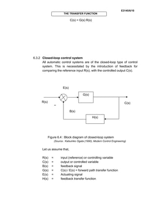
14. E3145/6/14
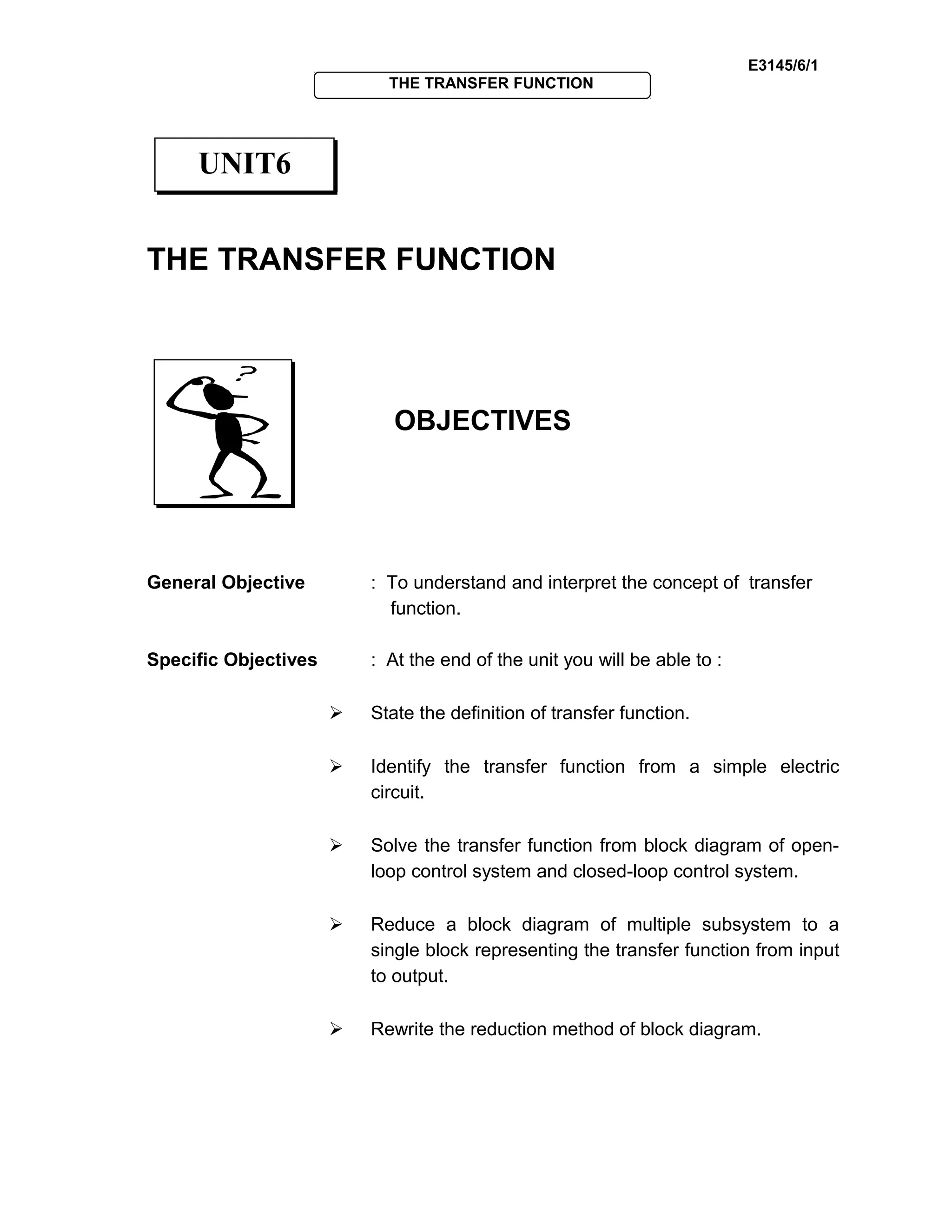
THE TRANSFER FUNCTION
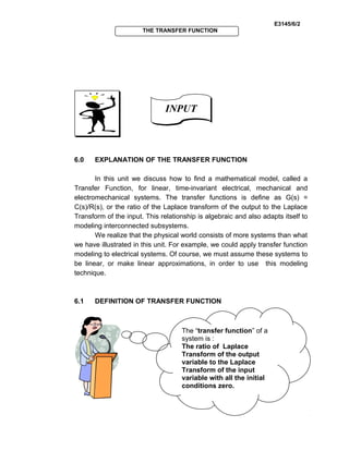
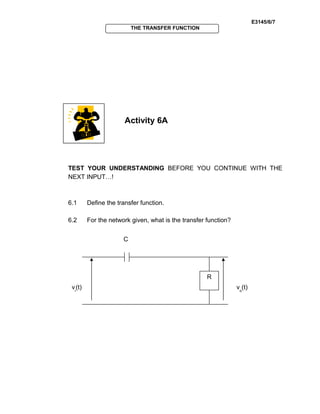
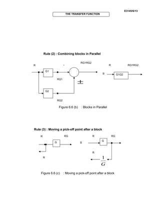
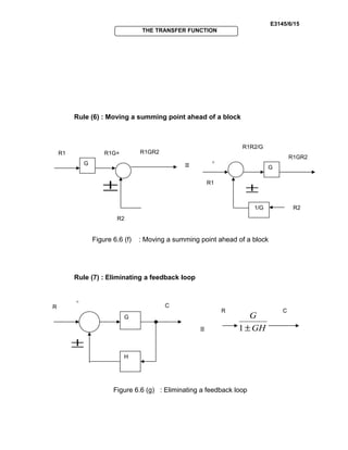
Rule (4) : Moving a take-off point ahead of a block
≡
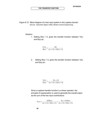
Figure 6.6 (d) : Moving a take-off point ahead of a block
Rule (5) : Moving a summing point after a block
≡
Figure 6.6 (e) : Moving a summing point after a block
R
G
RG
RG
G
G
RG
RG
R
R1
R2
R1R2
G
G[R1R2]
G
R1
+
R1G+
G
±
G[R1R2]
R2G
R2
±

15. E3145/6/15
THE TRANSFER FUNCTION
Rule (6) : Moving a summing point ahead of a block
≡
Figure 6.6 (f) : Moving a summing point ahead of a block
Rule (7) : Eliminating a feedback loop
≡
Figure 6.6 (g) : Eliminating a feedback loop
R2
R1R2/G
G
R1GR2
+G
R1 R1G+
±
R1GR2
R2
±
1/G
R1
G
H
R
±
+
C
R
GH
G
±1
C

16. E3145/6/16
THE TRANSFER FUNCTION
Figure 6.6 (a,b,c,d,e,f,g) : Block diagram reduction rules
(Source : Katsuhiko Ogata (1990), Modern Control Engineering)
6.3.4 A Block Diagram Reduction
The block diagram of a multiple-loop feedback control system is
shown in Figure 6.6. Use block diagram reduction to simplify this to a single
block relating C(s) to R(s). Note that, for clarity, the dependency upon s has
been omitted from the transfer functions within the blocks.
Figure 6.7 Block Diagram
G1
(s) G2
(s) G3
(s)
C(s)
H1
(s)
H2
(s)
H3
(s)
R(s) +
+_ _
+
+

17. E3145/6/17
THE TRANSFER FUNCTION
(a)
(b)
+
G1
(s) G3
(s)G2
(s)
H3
(s)
H2
(s)
H1
(s)
R(s) C(s)
- -
G1
(s) G2
(s)G3
(s)
H1
(s)H2
(s)H3
(s)
R(s) C(s)
-
+

18. E3145/6/18
THE TRANSFER FUNCTION
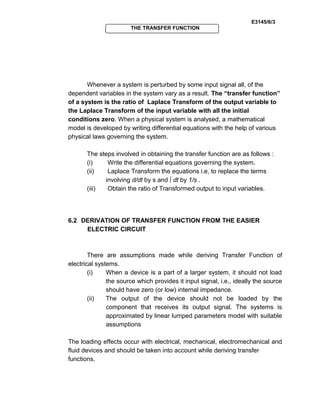
(c)
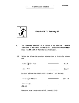
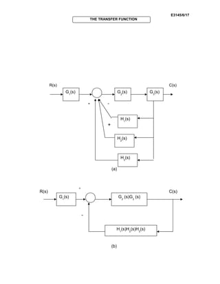
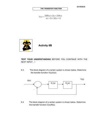
Figure 6.8 (a,b,c) : Steps to reduce the block diagram
(Source : Katsuhiko Ogata (1990), Modern Control Engineering)
Steps to reduce the block diagram :
(Figure6.8(a)) collapse summing junctions;
(Figure6.8(b)) form equivalent cascaded system in the forward
path and equivalent parallel system in the
feedback path;
(Figure6.8(c)) form equivalent feedback system and multiply by
cascaded G1(s)
Finally, the feedback system is reduced and multiplied by G1(s) to
yield the equivalent transfer function shown in Figure 6.7 (c ).
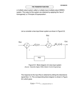
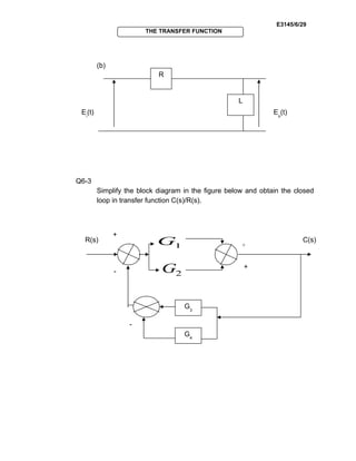
6.3.5 Block Diagram of Two Input System
In the present of more than one input to a system, the system may be
a single output system called a multiple-input-single-output (MISO) system or
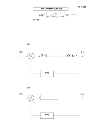
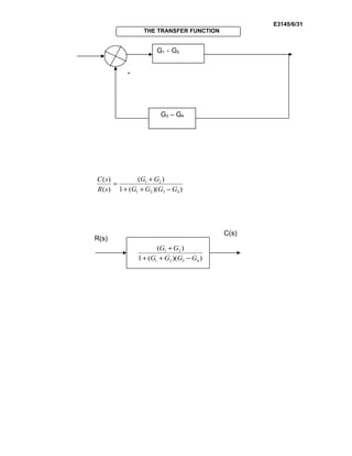
[ ])()()()()(1
)()()(
32132
123
sHsHsHsGsG
sGsGsG
+−+
R(s) C(s)

19. E3145/6/19
THE TRANSFER FUNCTION
a multiple output system called a multiple-input-multiple-output (MIMO)
system. The output of the system are obtained by applying the ‘law of
homogeneity’ or ‘Principle of Superposition’.
Let us consider a two-input linear system as shown in Figure 6.9.
Figure 6.9 : Block diagram of a two-input system
(Source : Katsuhiko Ogata (1990), Modern Control Engineering)
The response to the input R(s) is obtained by letting the disturbance
signal D(s) = 0. The corresponding block diagram is shown in Figure
6.9, which gives
CR(s) = )(
)( sR
sC acting alone with D(s) = 0
D(s)
_
)(1 sG )(2 sG
H(s)
R(s) C(s)

20. E3145/6/20
THE TRANSFER FUNCTION
CR(s) = 





+ )()()(1
)()(
21
21
sHsGsG
sGsG
R(s)
(6.3.4)
(a)
(b)
)(1 sG )(2 sG
H(s)
R(s) CR
(s)
-
H(s)
R(s) CR
(s)
-

21. E3145/6/21
THE TRANSFER FUNCTION
(c)
Figure 6.10(a,b,c) : Block Diagram Reduction with R(s) alone.
(Source : Katsuhiko Ogata (1990), Modern Control Engineering)
Similarly the response to the disturbance signal D(s) is obtained by
assuming R(s) = 0. The block diagram for this case is shown in Figure
6.11, which gives
CD(s) = )(
)( sD
sC acting alone with R(s) = 0
CD(s) = 





+ )()()(1
)(
21
2
sHsGsG
sG
D(s)
(6.3.5)
The actual response of the system when both R(s) and D(s) are acting
is obtained by adding the two individual responses CR(s) and CD(s).
)()()(1
)()(
21
21
sHsGsG
sGsG
+
R(s)
CR
(s)

22. E3145/6/22
THE TRANSFER FUNCTION
(a)
(b)
)(2 sG
G1
(s) H(s)
D(s) CD
(s)
-
H(s)
D(s) CD
(s)
-
G1
(s)

23. E3145/6/23
THE TRANSFER FUNCTION
(c)
Figure 6.11 (a,b,c) : Block Diagram Reduction with D(s) alone.
(Source : Katsuhiko Ogata (1990), Modern Control Engineering)
This example shows how superposition may be used to handle
system with more than one input :
Example 6.3: Determine the output Y(s) in the system shown below.
3+s
K
s
2
S + 1
R(s)
D(s)
Y(s)
-
+
+ +
)()()(1
)(
21
2
sHsGsG
sG
+
D(s)
CD
(s)

24. E3145/6/24
THE TRANSFER FUNCTION
Figure 6.12 : Block diagram of a two input system in the Laplace domain
(Source : Katsuhiko Ogata (1990), Modern Control Engineering)
Solution :
1. Setting D(s) = 0, gives the transfer function between Y(s)
and R(s) as :
)1(2)3(
2
)(
)(
+++
=
sKss
K
sR
sY
2. Setting R(s) = 0, gives the transfer function between Y(s)
and D(s) as :
)1(2)3(
)3(2
)(
)(
+++
+
=
sKss
s
sD
sY
Since a Laplace transfer function is a linear operator, the
principle of superposition is used to generate the overall output
as the sum of the two input contributions:
)1(2)3(
)()3(2
)1(2)3(
)(2
)(
+++
+
+
+++
=
sKss
sDs
sKss
sKR
sY
or

25. E3145/6/25
THE TRANSFER FUNCTION
)1(2)3(
)()3(2)(2
)(
+++
++
=
sKss
sDssKR
sY
Activity 6B
TEST YOUR UNDERSTANDING BEFORE YOU CONTINUE WITH THE
NEXT INPUT…!
6.3 The block diagram of a certain system is shown below. Determine
the transfer function Y(s)/U(s).
6.4 The block diagram of a certain system is shown below. Determine
the transfer function C(s)/R(s).
G1
(s) G2
(s)
U(s)
-
Y(s)

26. E3145/6/26
THE TRANSFER FUNCTION
Feedback To Activity 6B
6.3
)(
)(
sU
sY
=
)()(1
)()(
21
21
sGsG
sGsG
+
6.4
)(
)(
sR
sC
=
)(1
)(
sG
sG
+
G(s)
R(s)
-
C(s)

27. E3145/6/27
THE TRANSFER FUNCTION
KEY FACTS
1. The transfer functions is define as G(s) = C(s)/R(s), or the ratio of the
Laplace transform of the output to the Laplace Transform of the input.

28. E3145/6/28
THE TRANSFER FUNCTION
SELF-ASSESSMENT
You are approaching success. Try all the questions in this self-assessment
section and check your answers with those given in the Feedback on Self-
Assessment given on the next page. If you face any problems, discuss it
with your lecturer. Good luck.
Q6-1 State the steps to obtain the transfer function.
Q6-2
(a) The transfer function E0(s)/E1(s) of the RC-network shown is
given by:
Eo
(t)Ei
(t)
R
C

29. E3145/6/29
THE TRANSFER FUNCTION
(b)
Q6-3
Simplify the block diagram in the figure below and obtain the closed
loop in transfer function C(s)/R(s).
Eo
(t)Ei
(t)
R
L
2G
1G
G4
R(s) C(s)
G3
-
+
+
+
-

30. E3145/6/30
THE TRANSFER FUNCTION
Feedback To Self-Assessment
Have you tried the questions????? If “YES”, check your answers now.
Q6-1 The steps involved in obtaining the transfer function are as follows :
(i) To write the differential equations governing the system.
(ii) To Laplace Transform the equations i.e, to replace the terms
involving d/dt by s and ∫ dt by 1/s .
(iii) To obtain the ratio of Transformed output to input variables.
Q6-2 (a)
1
1
)(
)(0
+
=
RCssE
sE
i
(b)
LsR
Ls
sE
sE
i +
=
)(
)(0
Q6-3
R(s) C(s)

31. E3145/6/31
THE TRANSFER FUNCTION
))((1
)(
)(
)(
4321
21
GGGG
GG
sR
sC
−++
+
=
))((1
)(
4321
21
GGGG
GG
−++
+
G1 + G2
G3 – G4
-
R(s)
C(s)