This document describes the implementation of an Extended Kalman Filter (EKF) to estimate the state (position and heading angle) of a bicycle model. The EKF was able to provide reasonably accurate estimates of position over time based on position measurements and steering/velocity inputs, but struggled to accurately estimate the heading angle due to a lack of direct measurements. Histograms of the final state errors across many test cases showed normally distributed position errors and a uniformly distributed random heading angle error. While the EKF provided an approximation, a more advanced filter may have yielded better heading angle estimates.

1. ME231B/EE220C: Programming Project
Muireann Spain
4th May 2020

2. Contents
1 Prior . . . . . . . . . . . . . . . . . . . . . . . . . . . . . . . . 2
2 Introduction . . . . . . . . . . . . . . . . . . . . . . . . . . . . 3
3 Estimator Selection and Design . . . . . . . . . . . . . . . . . 5
4 Results . . . . . . . . . . . . . . . . . . . . . . . . . . . . . . . 8
5 Conclusion . . . . . . . . . . . . . . . . . . . . . . . . . . . . . 12
1

3. 1 Prior
All edited code was completed in MATLAB and can be found in the
accompanying Gradescope submission.
The below work references both the project brief provided for this project
and Chapter 10: The Extended Kalman Filter in the accompanying course
notes.
2

4. 2 Introduction
The problem specified required the implementation of a state estimator
that tracks the X-coordinate, Y-coordinate and heading angle of a bicycle.
Figure 1 was provided in the project brief, and illustrates the system
model. X1(t) and Y1(t) are the X- and Y- coordinates of the rear wheel, B
is the wheelbase (m), γ(t) is the steering angle relative to the bicycle
frame, θ(t) is the heading angle and ω(t) is the angular velocity of the rear
wheel.
Figure 1: Simple Bicycle Model Used
The bicycle dynamics were predefined as follows:
˙x1(t) = v(t) cos (θ(t)) (1)
˙y1(t) = v(t) sin (θ(t)) (2)
˙θ(t) =
v(t)
B
tan (γ(t)) (3)
where v(t) is the linear velocity of the bicycle.
3

5. An idealized measurement model p(k) of the discretized position
coordinates was also specified in the project brief:
p(k) =
x1(tk) + 1
2
B cos (θ(tk))
y1(tk) + 1
2
B sin (θ(tk))
(4)
It is known that measurements are obtained approximately every 0.5
seconds, however the sensors are faulty and measurements are not
guaranteed. γ(t) and ω(t) are known with certainty at each time step.
The goal is to design an estimator that can minimize the error in the
prediction of the true position and heading angle of the bicycle at the final
time step.
4

6. 3 Estimator Selection and Design
This project was completed in MATLAB. The Extended Kalman Filter
(EKF) was chosen as an acceptable estimator for this project. The EKF
functions by linearizing the system equations about the current state
estimate, and applying a standard Kalman Filter prior and measurement
update equations to the linearized equations.
In this system, three states were defined for estimation: the X-coordinate
X, the Y-coordinate Y and the heading angle θ.
As shown above in Section 2, the bicycle dynamics were given in terms of a
continuous time model. The state space was discretized at Ts = 0.25s, as
the EKF equations are applied at discrete time intervals - although
measurements are obtained at approximately every 0.5 s, I found 0.25 s to
be optimal. The MATLAB inbuilt state-space model from the control
toolbox was used for this purpose. 1
The continuous time model was specified as follows, and are obtained from
linearizing the system equations about the current state estimate (which
depends on real-time measurements):
A(k) =


1 + v(t) cos (θ(k)) 0 0
0 1 + v(t) sin (θ(k)) 0
0 0 1 + v(t)
B
tan (γ(k))

 (5)
B(k) =


0 0
0 0
0 0

 (6)
H(k) =
1 0 −0.5B sin (θ(k))
0 1 0.5B cos (θ(k))
(7)
1
Interestingly, I accidentally initially used the continuous model in place of the dis-
cretized model, and I actually obtained superior performance from the estimator. How-
ever, this approach is clearly incorrect, and so I sacrificed estimator performance for
modelling accuracy. I am also unable to explain and justify this behaviour!
5

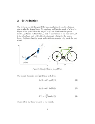
7. D(k) =
0 0
0 0
(8)
The matrices L(k), M(k) are obtained from the process noise derivative of
the state equation and measurement noise derivative of the measurement
equation respectively. As the process noise
For this system, these matrices are defined as follows:
L(k) =


1 0 0
0 1 0
0 0 1

 (9)
M(k) =
1 0
0 1
(10)
In this case, the position is measured and the heading angle is estimated.
However, given that the position measurements were not guaranteed at
each time step, a contingency was introduced to provide a measurement
estimate from the idealized model specified in Equation 4. When no
real-time measurements were provided, the position update was estimated
by Equation 11, in which α is a random variable in the range [0, 1] which
serves the purpose of added uniform noise.
z(k) =
0.99(x1(tk) + 1
2
B cos (θ(tk))) + 0.01α(x1(tk) + 1
2
B cos (θ(tk)))
0.99(y1(tk) + 1
2
B sin (θ(tk))) + 0.01α(y1(tk) + 1
2
B sin (θ(tk)))
(11)
There were certain other parameters that were defined to meet the
Extended Kalman Filter equation requirements:
V : approximation of the process noise variance,
W: approximation of the measurement noise variance, and
Pm: approximation of the prior conditional variance of the initial states
X,Y and θ.
The values for these parameters are shown in Equations 12, 13 and 14.
These values were converged upon by trial and error measuring the mean
6

8. and variance of the final error over all 93 data sets. However, the drastic
altering of these values did not have a huge impact on the final estimation
error.
V =


10 0 0
0 10 0
0 0 0.1

 (12)
W =
0.05 0
0 0.05
(13)
Pm =


10 0 0
0 10 0
0 0 0.1

 (14)
7

9. 4 Results
The output of the main() MATLAB function is illustrated in Figure 2 and
Figure 3 for two randomly selected data sets. It can be seen graphically for
both cases that the estimator appears to have a decent approximation of
both the X- and Y- coordinates appear to follow the path in both cases.
The approximation of the heading angle θ is very inaccurate in both data
sets and oscillates significantly which does not represent the true heading
angle.
Figure 2: Estimator Performance For First Data Set
Figure 3: Estimator Performance For 78th Data Set
8

10. Histograms illustrating the mean and variance of X, Y and θ are shown in
Figures 4, 5 and 6 respectively. This data was obtained by measuring the
final error over all 93 data sets. The observations of these histograms
quantify what was roughly observed from the graphs in Figure 2 and 3.
The position errors are normally distributed, however both resulting errors
have a positive bias of approximately 0.2 m. The distribution of the Final
X-coordinate error has a tighter variance than the Y-coordinate equivalent.
Figure 4: Histogram of Heading Angle Error at Final Position
9

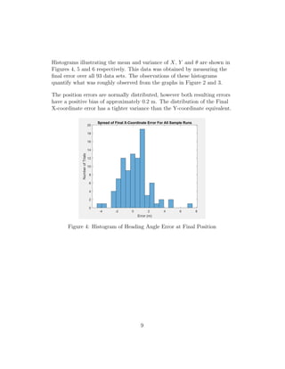
11. Figure 5: Histogram of Heading Angle Error at Final Position
The distribution of the final heading angle error, however, is uniform and
random. Given that the range of possible values of θ is [−π, π], the
estimator does not estimate the heading angle with any precision. This
may be because no measurements of heading angle are received, and the
value of θ is initialized as π
2
, as it is stated in the project brief that the
cyclist is headed ”approximately North-East” for each of the test cases.
10

12. Figure 6: Histogram of Heading Angle Error at Final Position
11

13. 5 Conclusion
As stated in the course notes, if the actual state and noise values are close
to the values that we linearize about, then the linearization is a good
approximation of the actual nonlinear dynamics. The underlying
assumption we make, when using the EKF, is that we can push a random
variable through a linear function and use the linearization to compute the
resulting random variable’s statistics.
In the case of Gaussian noise, these quantities are not guaranteed to be
small since the noise is actually unbounded.
The EKF provides only an approximation of the conditional mean and
variance, and not the true value. In the case of this bicycle system,
significant effort was made to tune the parameters V , W, Pm(0) along
with the initial conditions of the state. This tuning resulted in little
reduction of the variance of the final error of the state estimation. The
EKF can be applied in this system, as the simplified bicycle dynamics are
not extremely nonlinear and the distribution is unimodal. The use of a
simplified model and the lack of measurement data for each time step
result in added uncertainty of estimation.
However, in hindsight the Unscented Kalman Filter or the Particle Filter
would probably provide a more accurate state estimation of this system’s
true final position.
12