DC Motor Modelling & Design Fullstate Feedback Controller

Name : IB.P.P.Mahartana
NRP : 2111100177

DC MOTOR STATESPACE CONTROL
1. Full-state Feedback Controller DC motor Speed.
A. Mathematical Model of DC motor
A common actuator in control systems is the DC motor. It directly provides
rotary motion and, coupled with wheels or drums and cables, can provide
translational motion. The electric circuit of the armature and the free-body
diagram of the rotor are shown in the following figure 1.1:
Figure 1.1 Mathematical Model Dc motor.
(http://ctms.engin.umich.edu)
For this project the following values for the physical parameters already
knowns and listed in tabel 1.1.
Tabel 1.1 Physical Dc motor parameters.
No Parameters Unit
1 Moment of Inertia of the rotor (J) 0.01 kg.m2
2 Motor viscous fricttion constant (b) 0.1 N.m.s
3 Electromotive force constant (Ke) 0.01 V/rad/sec
4 Motor torque constant (Kt) 0.01 N.m/Amp
5 Electrical resistance (R) 1 Ohm
6 Electircal Inductance (L) 0.5 H

B. Drive The Equation motion of the system.
B.1 FBD Electrical System.
Figure 1.2 FBD Electrical System
𝑇𝑒 = 𝐾∅𝑖 = 𝐾𝑡 𝑖 Electromagnectic Torque
𝑒 = 𝐾∅𝜔 = 𝐾𝑒 𝜃̇ Armature back e.m.f
𝐿 𝑎
𝑑𝑖
𝑑𝑡
= −𝑅𝑖 + 𝑉 − 𝑒
B.2 FBD Mechanical System
∑ 𝑀 = 0
𝐽
𝑑2
𝜃
𝑑𝑡2
= 𝑇𝑒 − 𝑏
𝑑𝜃
𝑑𝑡

C. Drive State-space model of the system
Total Equation Motion of the system :
𝑑2
𝜃
𝑑𝑡2
=
1
𝐽
(𝐾𝑡 𝑖 − 𝑏
𝑑𝜃
𝑑𝑡
)
𝑑𝑖
𝑑𝑡
=
1
𝐿
(−𝑅𝑖 + 𝑉 − 𝐾𝑒
𝑑𝜃
𝑑𝑡
)
The state-space model have the standard form shown below where the
state vector x = 𝜃𝑖̇ and the input for the system is u = V, and the output velocity
which is thetha_dot will be my output desire.
𝑥 = 𝐴𝑥 + 𝐵𝑢
𝑦 = 𝐶𝑥 + 𝑑𝑢
̇
𝑥 =
𝑑
𝑑𝑡
[ 𝜃̇
𝑖
] =
[
−
𝑏
𝐽
𝐾
𝐽
−
𝐾
𝐿
−
𝑅
𝐿]
[ 𝜃̇
𝑖
] + [
0
1
𝐿
] 𝑉
𝑦 = [1 0] [ 𝜃̇
𝑖
]
D. Simulink Model without control
Figure 1.3 Open Loop system Simulink diagram block

E. Matlab Commands.
% Define motor Parameters
J = 0.01; % Moment Inertia of the rotor
b = 0.1; % Motor viscous friction constant
K = 0.01; % Electromotive force constant,motor torque
constant
R = 1; % Electrical Resistance
L = 0.5; % Electrical Inductance
% Define motor state variable model
A = [-b/J K/J;-K/L -R/L];
B = [ 0;1/L ];
C = [ 1 0 ];
D = 0;
plot(t,y,'g','linewidth',2);
xlabel('time in second');
ylabel('Angular Velocity (rad/s)');
title('Step respon for Open Loop System');
grid on
F. Plotted result of open loop system
Figure 1.4 Step respon plot for Open loop system

By using stepinfo command below, we obtain the performances of the openloop
system.
%Obtain Open-loop Performance
S = stepinfo(sys)
And the result are:
S =
RiseTime: 1.1351
SettlingTime: 2.0652
SettlingMin: 0.0899
SettlingMax: 0.0998
Overshoot: 0
Undershoot: 0
Peak: 0.0998
PeakTime: 3.6758
As you can see , when the system was given an input voltage about 1 Volt, the
motor can only achieved the maximums angular speed about 0.1 rad/sec and
become stable at 3 second, the system has a large steady state error when the final
value of the step input reference was given by default 1 rad/s.
G. Designing the full-stateback controller
Full state feedback (FSF), or pole placement, is a method employed in feedback
control system theory to place the closed-loop poles of a plant in pre-determined
locations in the s-plane. Placing poles is desirable because the location of the poles
corresponds directly to the eigenvalues of the system, which control the
characteristics of the response of the system.
Figure 1.5 Closed Loop Full state feedback controller in state-space model

G.1 Design Criteria
For a 1-rad/sec step reference, the design criteria are shown in table 1.2
Table.1.2 Design criteria
G.2 Simulink Block Diagram
The Simulink block diagram are used to get the model and design the pole
placement controller with goal to achieved the design criteria.
Figure 1.6 Simulink Block Diagram State-feedback Controller DC motor.
First Statespace block contains the initial state and output matrix of Dc motor and
the second statespace block contains the estimator matrix where the feedback
matrix came in the form look like this sI - (A - B*Kc) here s is the Laplace variable.
Since the matrices A and B*Kc are both 2x2 matrices, there should be 2 poles for
the system. To eliminate the steady state error we need to adding precompensator
. It could be done by simply using rscale function in matlab command, but in this
project we’ve using gain by the value of ten, so that the output in turn is scaled to
the desired level.
Settling time < 2 second
Overshoot < 5%
Steady-state error < 1%

G.3 Matlab Source-Code
Before running the simulink file, the matlab command to define all the parameters
must be done.
J = 0.01; % Moment Inertia of the rotor
b = 0.1; % Motor viscous friction contant
K = 0.01; % Electromotive force constant, motor torque constant
L = 0.5; % Electrical Inductance
A = [-b/J K/J;-K/L -R/L]
B = [ 0;1/L ]
C = [ 1 0 ]
D = [ 0]
% check observability
O = obsv(A,C)
rank(O)
% Obtain feedback gain by placing 2 poles with vary value
p1 = -7; % Change based on table 1.3
K = acker(A,B,[p1 p2])
% Define the Estimator statespace
Aes= A-B*K % Change matrix A , the rest still same
sys=ss(Aes,B,C,D);
% plot the root locus
subplot(2,1,1);
pzmap(sys)
% Plotting State Respon with State-Feedback controller
Uncontrolled_system = un;
With_state_feedback = con;
subplot(2,1,2);
plot
(t,Uncontrolled_system,'r',t,With_state_feedback,'b','linewidth',2
);
xlabel('Time in second');
ylabel('Amplitude (rad/s)');
title ('State Respon Uncontrolled VS State-feedback controller')
legend ('Uncontrolled system','With state feedback');
grid on
hold off
% Obtain the system performances
S= stepinfo(con,t)

G.4 Vary pole location
To know how the system behave cause of changing of the poles value, we need to
try several poles value. Table 1.3 shown vary poles location.
Table 1.3 Vary poles location
Type of poles Poles 1 Poles 2
Real number same
value
-7 -7
Real number different
value
-6.5 -4.35
Complex number -5+1.5i -5-1.5i
Complex number -3+3.5i -3-3.5i
G.4.1 System respon.
1. The root locus and respon for twin pole (±7) in the real part
Figure 1.7 Root locus and respon with poles place at (±7)

The system has performance shown below:
2. The root locus and respon of differents poles (-6.5 and -4.35) in the real part.
Figure 1.8 Root locus and respon with poles place at (-6.5 and -4.35)
Settling time 0.8359s
Overshoot 0
Steady-state error <1%
Rise time 0.4804
Peak time 3
Settling time 1.1417
Overshoot 0
Rise time 0.6523
Peak time 3

3. The root locus and respon of complex poles (-5±1.5i)
Figure 1.9 Root locus and respon with poles place at (-5±1.5i)
Overshoot 0.0027
Rise time 0.6069
Peak Time 2.1252

The root locus and respon of complex poles (-3±3.5i)
Figure 1.9 Root locus and respon with poles place at (-3±3.5i)
Overshoot 6.711
Rise time 0.4347
Peak Time 0.9252

H. Analysis of poles location.
We’ve been simulate and plotted all the poles location in table 1.3 and the result
has shown above. The relationship between the pole location and the specification
of the system are demostrate by figure 1.20 below.
Figure 1.20 pole location in the s-plane
Since horizontal lines on the s-plane are lines of constant imaginary value, they’re
also lines of constant peak time, and the vertical lines on the s-plane are lines of
constant real value, they’re also the lines of constant settling time. As the poles
move in a horizontal direction either right or left, the real part has change and
keeping the imaginary part remain constant. This condition will change the setlling
time performance, as we can see from figure 1.7-1.9, we were changing the poles
location move to the right it caused the settling time performance increased. But at
figure 1.6-1.7 has the same peak time, it maked sense because the system weren’t
having any imajinary part, so the imajinary part remain the same.
Let us now figure out what happens at figure 1.8-19, obviously the system now has
imajinary part, since ζ =cosθ represent overshoot and as we move the poles in
vertical direction its increasing the overshoots because its change the radial position
of θ.

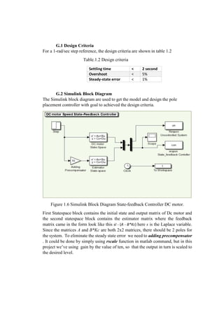
2. Full-state Feedback+ Integrall Controller DC motor Angular Position.
We’ve been created speed controller for Dc motor where the output comes out
from the statespace matrix is velocity. Now we’ll considering controller for angular
position of the rotor. To do that, we take the same model as shown above but we
need some modification through the statespace matrix and the parameters listed in
table 1.4 below to get poper model.
Table 2.1 Phsiycal parameters for Dc motor
No Parameters Unit
1 Moment of Inertia of the rotor (J) 3.2284E-6 kg.m2
2 Motor viscous fricttion constant (b) 3.5077E-6 N.m.s
3 Electromotive force constant (Ke) 0.0274 V/rad/sec
4 Motor torque constant (Kt) 0.0274 N.m/Amp
5 Electrical resistance (R) 4 Ohm
6 Electircal Inductance (L) 2.75E-6 H
A. Drive the state space model for the system
From the main problem, the dynamic equations in state-space form are given below.
𝑑
𝑑𝑡
[
𝜃
𝜃̇
𝑖̇
] =
[
0 1 0
0 −
𝑏
𝐽
𝐾
𝐽
0 −
𝐾
𝐿
−
𝑅
𝐿]
[
𝜃
𝜃̇
𝑖̇
] + [
0
0
1
𝐿
] 𝑉
𝑦 = [1 0 0] [
𝜃
𝜃̇
𝑖̇
]
For the initial respon from the system is pretty close the same with Dc motor speed
shown in sub section D until F with all we need just change the matrices
composition into 3x3 matrices and we good to go. The respon of uncotrolled system
shown in figure 1.21 below :

Figure 2.1 Respon the angular position of rotor without controller
As we can see, its seem like the amplitude of the angular position goes to the infinity
. The system performance listed below :
S =
Rise time : 0.0344 Settling time: 0.0493
Overshoot : 0 Peak time : 0.05
B. Designing the full-stateback controller
The control law for a full-state feedback system has the form u =r –K*x , the
characteristic polynomial for this closed-loop system os the derminant of sI-(A-
B*K) where s is the laplace variable, the associated block diagram is given by
figure1.5. Since the matrices of A and B*K are both 3x3 matices, it should be 3
poles exist in the system. Before we create the controller we need to verify our
system is controllable or not, by checking through the system order and its
deteminant. For this case the design criteria and the vary poles location has given
by table 2.1. and table 2.2
Table 2.1 Given Design Criteria with a 1-radian step reference
Settling time < 2 second
Overshoot < 5%
Steady-state error < 1%

Table 2.2 Vary poles location
C. Disturbance Respon
In order to observe the system’s disturbance response, we must provide the proper
input to the system. In this case, a disturbance will fit as a physically a load torque
that acts on the inertia of the motor. This load torque acts as an additive term in the
second state equation. We can simulate this by modifying our close-loop input
matrix, to have a 1/J in the second row what will act like our current input is only
the disturbance. We can perform this by define the B matrices in matlab command
below, so it can be use to simulate the whole system through our simulink file.
C.1 Simulink block Diagram
Figure 2.2 Dc motor position block diagram with feedback and disturbance
C.2 Matlab Source-Code
J = 3.2284E-6; % Moment Inertia of the rotor
b = 3.5077E-6; % Motor viscous friction contant
K = 0.0274; % Electromotive force constant, motor torque
L = 2.75E-6; % Electrical Inductance
Type of poles Poles 1 Poles 2 Pole 3
Real number same
value
-450 -450 -450
Real number different
value
-735 -567 -325
Complex number -255+50i -255-50i -100
Complex number -100+100i -100-100i -200

A = [0 1 0; 0 -b/J K/J; 0 -K/L -R/L]
B = [0 ; 0 ; 1/L]
C = [1 0 0]
D = [0]
% check observability and controllable
determinant = det(ctrb(A,B))
O = obsv(A,C);
rank(O)
% Obtain feedback gain by placing 3 poles with vary value
K = place(A,B,[p1, p2, p3])
% Modifying the close-loop input matrix B
F = A-B*K % state feed back A matrices
Bd = [0; 1/J ; 0] % Disturbance input matrices, the rest are still
same.
Disturbance = con;
plot (t,Disturbance,'linewidth',2 );
ylabel('Amplitude (rad)');
title ('Disturbance respon of rotor angular position')
grid on
S= stepinfo(con,t)

D. Plotted result for disturbance respon and vary poles location
1. The Disturbance and feedback respon when same poles place
at (-450)
Figure 2.3 Disturbance respon of rotor angular position
at poles location (-450)
The system performance listed below :
S =

2. The Disturbance and feedback respon when differents poles place
at (-735 -567 -325).
at poles location (-735 ,-567, -325).
S =

3. The Disturbance and feedback respon when complex poles place
at (-255+50i, -255-50i, -100).
at poles location (-255+50i, -255-50i, -100).
S =

4. The Disturbance and feedback respon when complex poles place
at (-100+100i, -100-100i -200).
at poles location (-100+100i, -100-100i, -200).
S =
Overshoot : 0 2.1132 Peak time : 0.00359
E. Adding integral action
Putting an extra integrator in series with the plant it can remove the steady-state
error due to a step reference. If the integrator comes before the injection of the
disturbance, it will also cancel a step disturbance input in steady state. the associated
block diagram is given by figure 2.4.

Figure 2.6 Associated block diagram for series adding integral with the plant
We can model the addition of this integrator by augmenting our state equations with
an extra state for the integral of the error which we will identify with the variable
w. This adds an extra state equation, where the derivative of this state is then just
the error, e = y - r where y = theta. This equation will be placed at the bottom of
our matrices. The reference r, therefore, now appears as an additional input to our
system. We’re gonna need to rebuilt the estimator block in figure 2.1 into
augmented block by implemented the new 4x4 matrices shown below.
The augmented additional integrator state are represent by matrices Aa, Ba, Ca and
Da. In order to find the closed-loop equations, all we need to do is to look at how
the step input, affects the plant. In this case, it affects the system in exactly the same

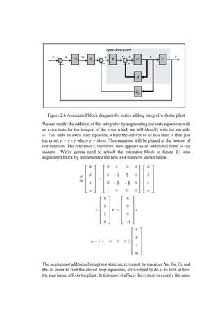
manner as in the unaugmented equations except now u = -Kc x - Ki w. We can also
rewrite this in terms of our augmented state as u = -Ka xa where Ka = [ Kc Ki ].
Substituting this u into the equations above provides the following closed-loop
equations.
𝑋̇ 𝑎 = (𝐴 𝑎 − 𝐵𝑎 𝐾𝑎)𝑥 𝑎 + 𝐵𝑟 𝑟
𝑦 = 𝐶 𝑎 𝑥 𝑎
As we can see the integral of the error will fed back again, then it would eliminate
the steady state error goes to zero. Since the augmented matrices has 4x4 form,it
should have 4 poles inside, moreover we need to adding fourth pole into the system
we will use -600.
E.2 Matlab Source-Code
We used the same simulink block in figure 2.2 then we change all the parameters
based on the matlab command below.
% Obtain augmented 4x4 state matrices Aa, Ba, Ca, Da
Aa = [0 1 0 0; 0 -b/J K/J 0 ; 0 -K/L -R/L 0; 1 0 0 0];
Ba = [0 ; 0 ; 1/L ; 0 ];
Br = [0 ; 0 ; 0; -1];
Ca = [1 0 0 0];
Da = [0];
% Obtain feedback gain by placing 4 poles and other poles same as
before
p1 = -100+100i;
p2 = -100-100i;
p3 = -200;
p4 = -600;
Ka = acker(Aa,Ba,[p1, p2, p3,p4])
% Define the augmanted statespace
G = Aa-Ba*Ka
H = Br
I = Ca
J = Da
integral = con;
plot (t,integral,'','linewidth',2 );
ylabel('Amplitude (rad)');
ylim([0 1.05]);
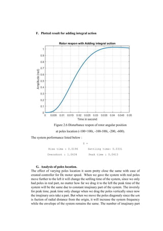
title ('Rotor respon with Adding integral action')
grid on
S= stepinfo(con,t)

F. Plotted result for adding integral action
at poles location (-100+100i, -100-100i, -200, -600).
S =
Overshoot : 1.0634 Peak time : 0.0413
G. Analysis of poles location.
The effect of varying poles location it seem pretty close the same with case of
created controller for Dc motor speed. When we gave the system with real poles
move further to the left it will change the setlling time of the system, since we only
had poles in real part, no matter how far we drag it to the left the peak time of the
system will be the same due to constant imajinary part of the system. The inversly
for peak time, peak time only change when we drag the poles vertically since now
the imajinary axis take a part. But when we move the poles diagonaly since the 𝜔𝑛
is fuction of radial distance from the origin, it will increase the system frequency
while the envelope of the system remains the same. The number of imajinary part

in poles also effect the overshoot of the system since the overshoot is a fuction of
zheta. Adding extra integral will remove the steady state error of the system,
obviously this could happens because when we add integral in series with the plant,
it change the whole system type. Since steady state-state error are depend upon the
number ontegration in the forward path. We already know, since we define the
system type to be the value of n in the denominator or eqivalently, the number of
pure integration in the forward path. Therefore,a system with n = 0 is a Type 0
system. If n = 1 or n = 2, the coressponding system is a type 1 or type 2 system.
Thats why when we adding integral the type of system change into type 1 or 2 when
we know the value of steady state error with step input u(t) would be zero.

DC Motor Modelling & Design Fullstate Feedback Controller

More Related Content

Similar to DC Motor Modelling & Design Fullstate Feedback Controller

Recently uploaded

DC Motor Modelling & Design Fullstate Feedback Controller