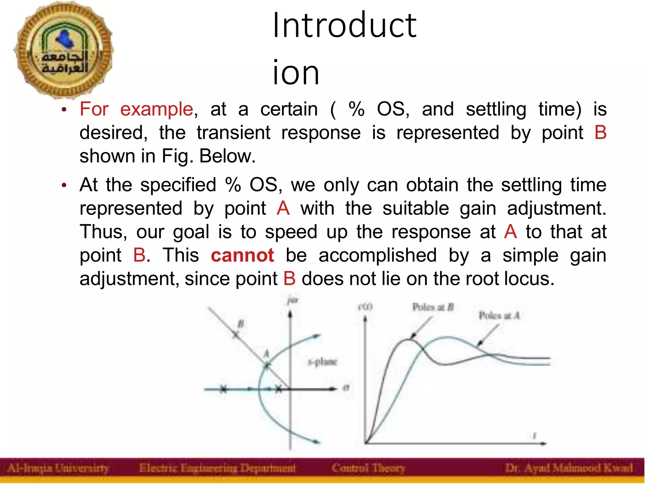
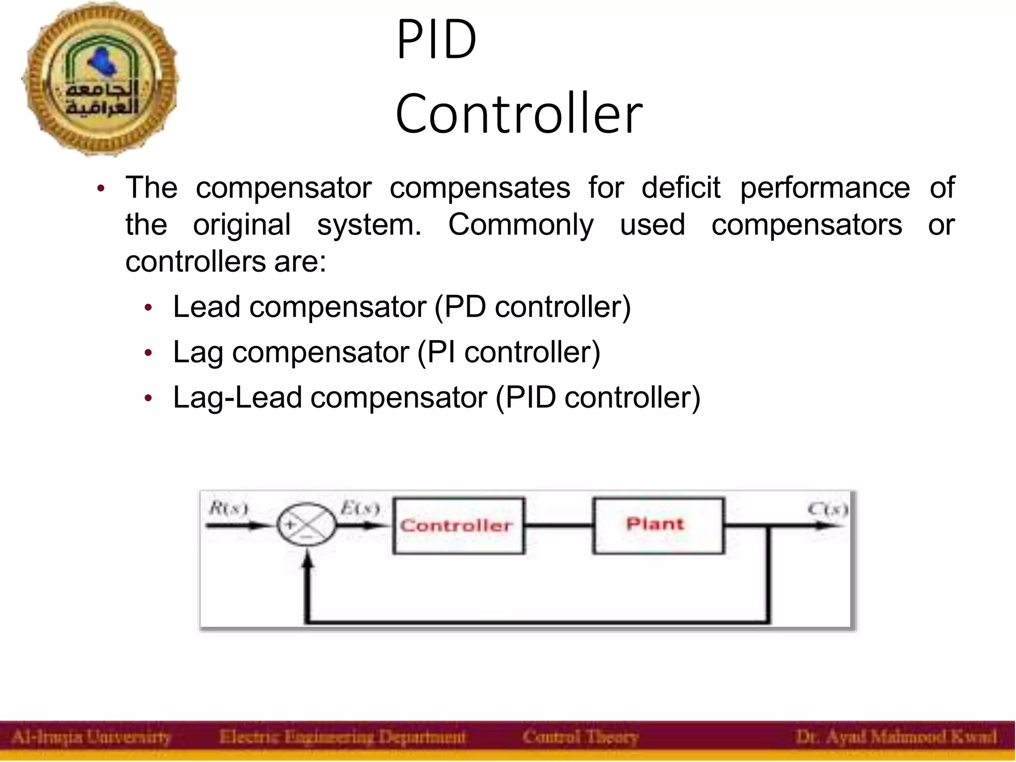
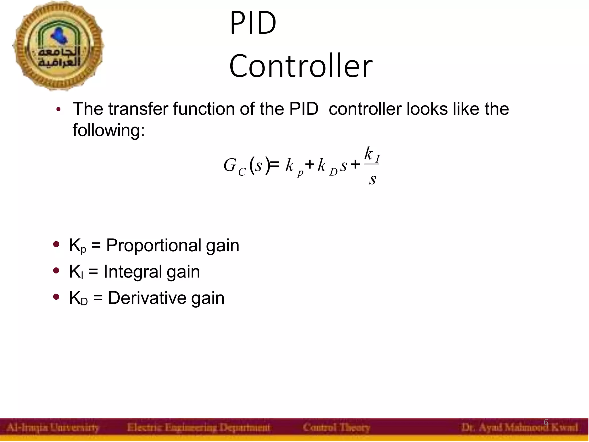
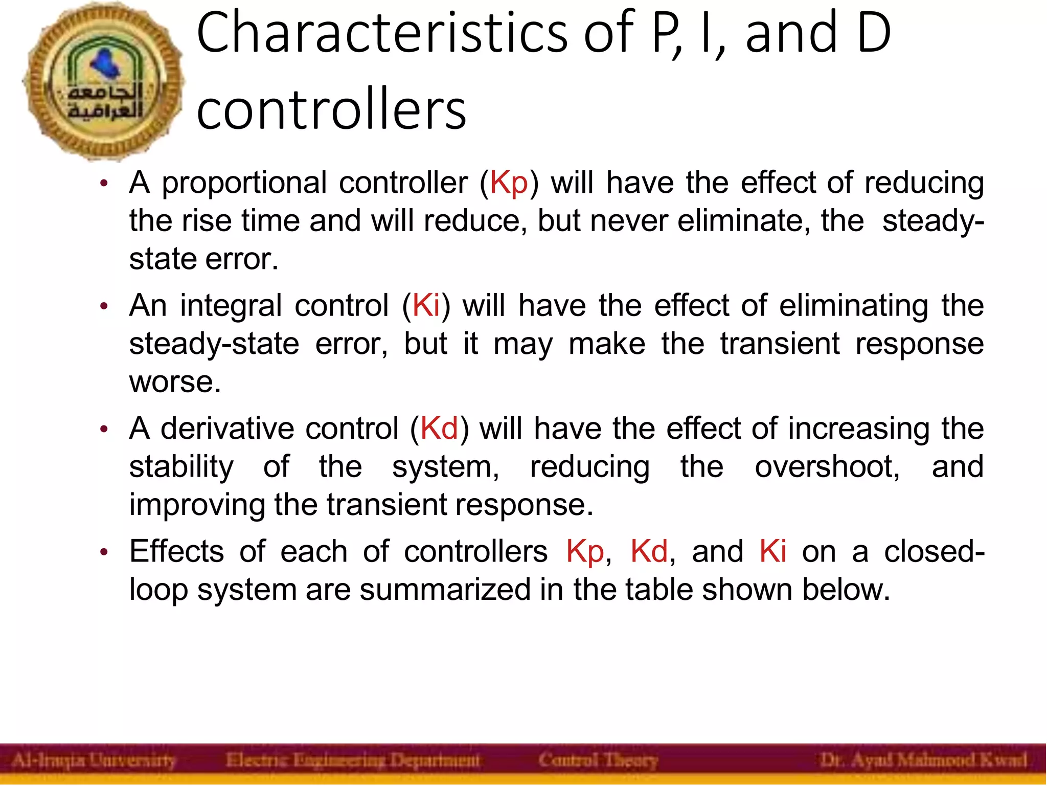
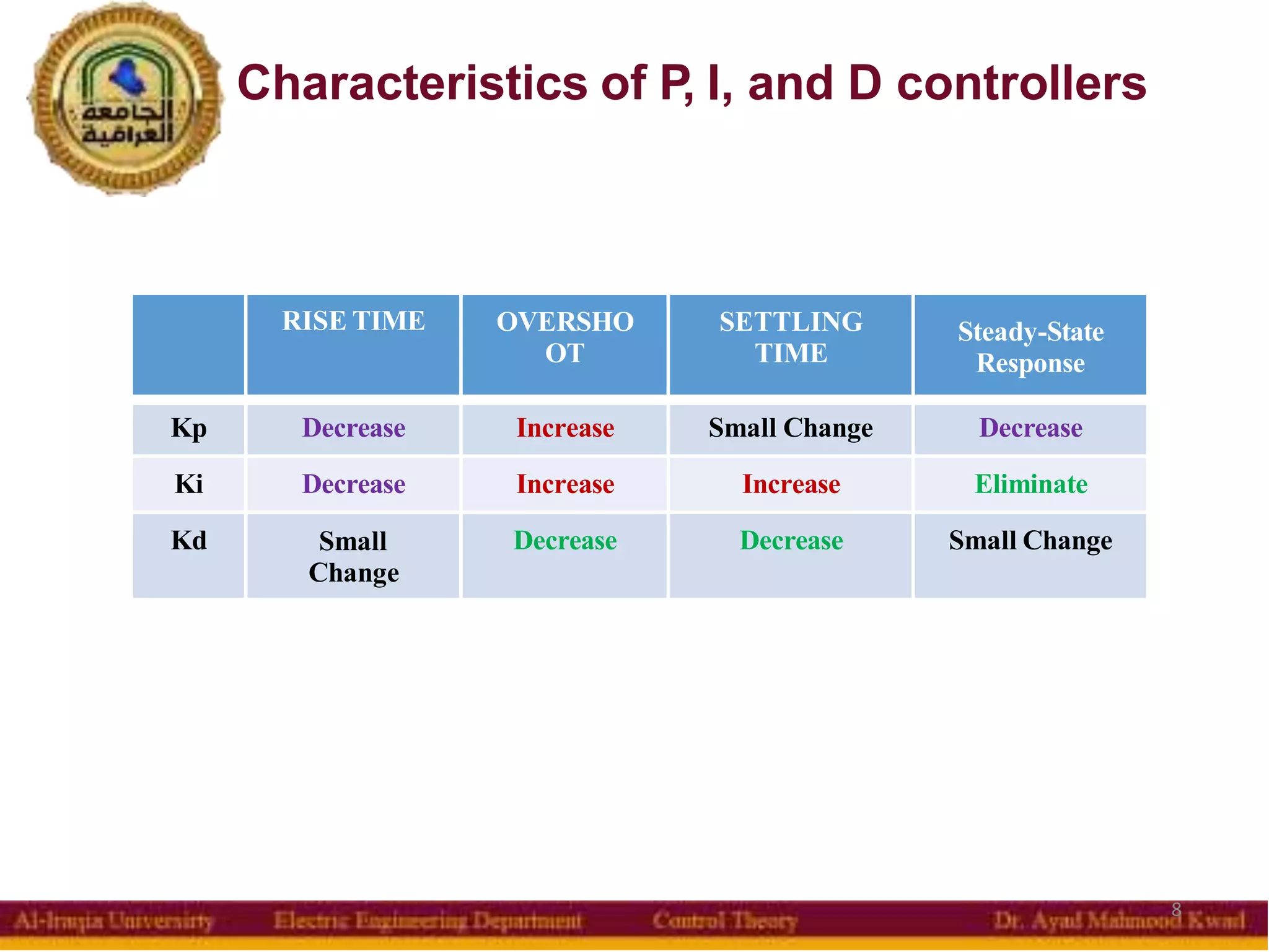
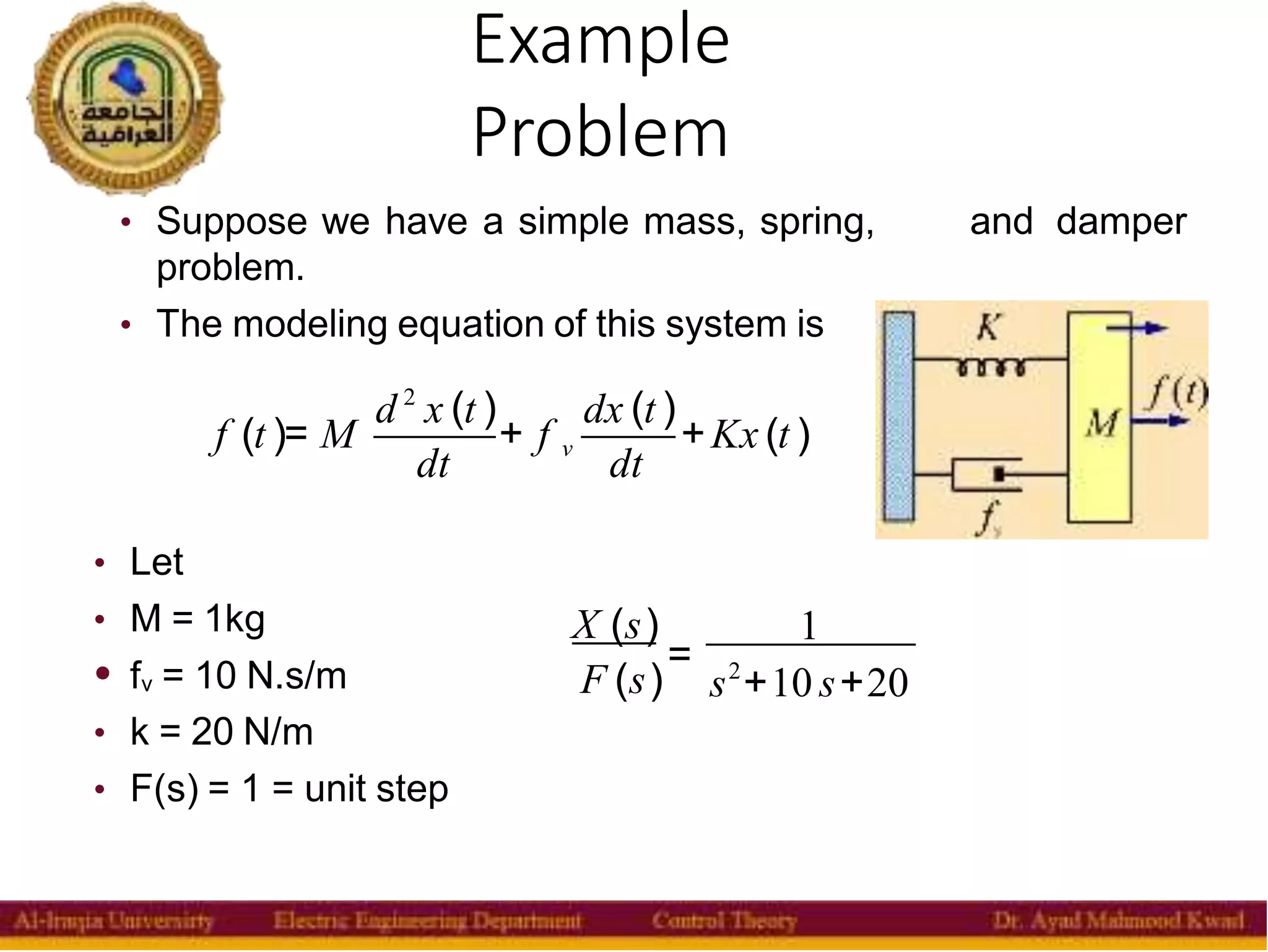
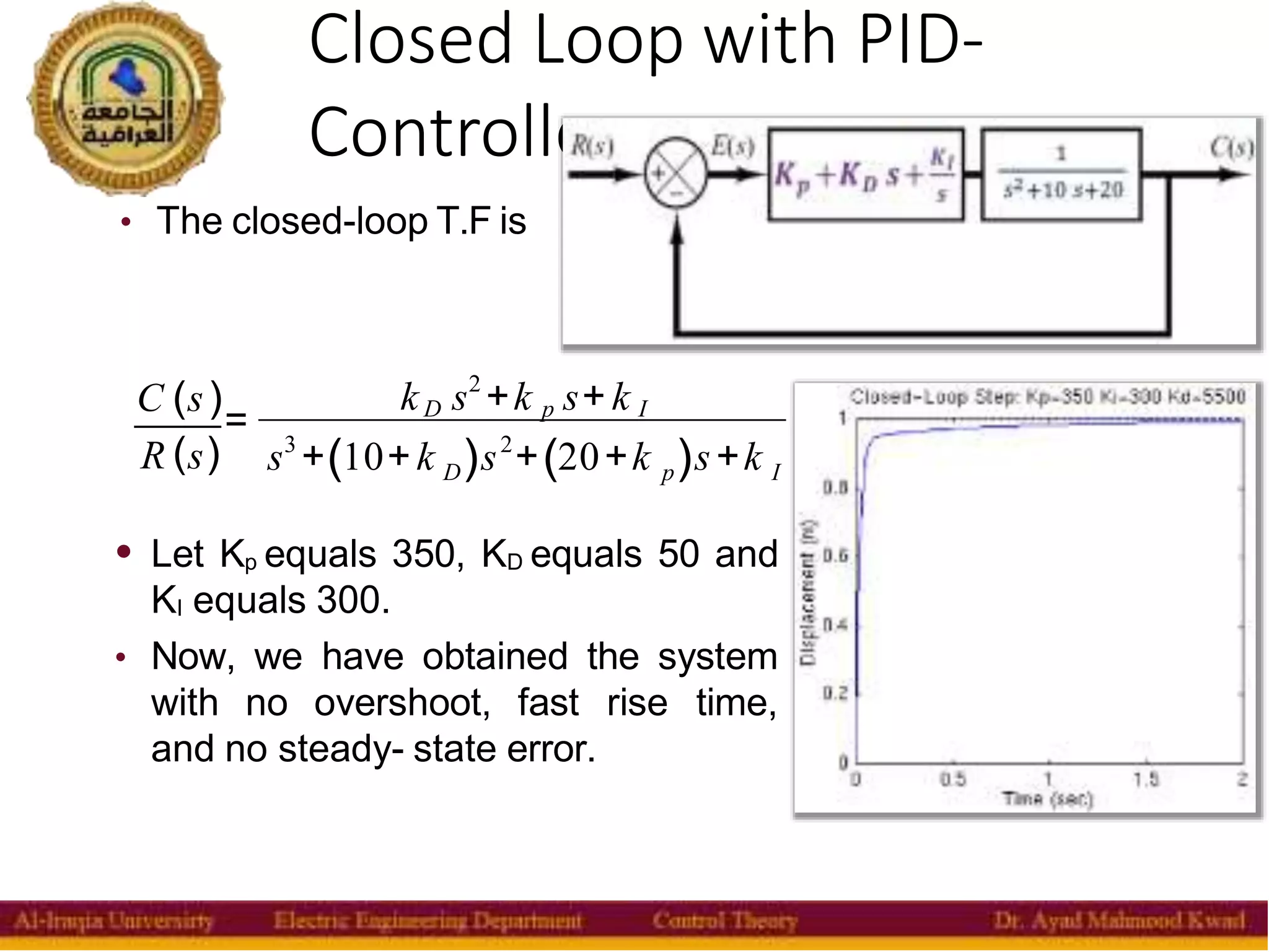
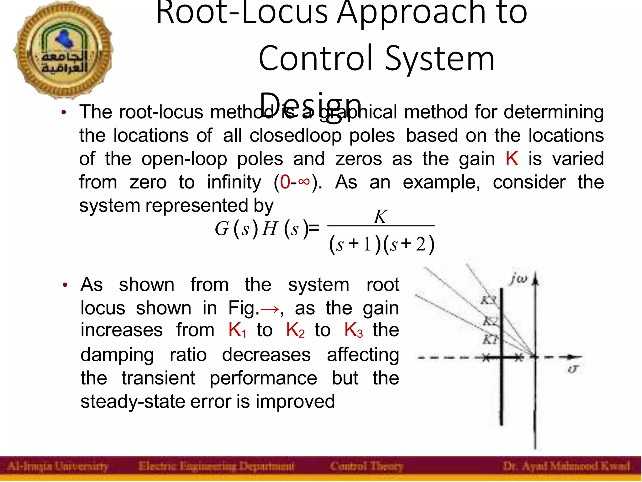
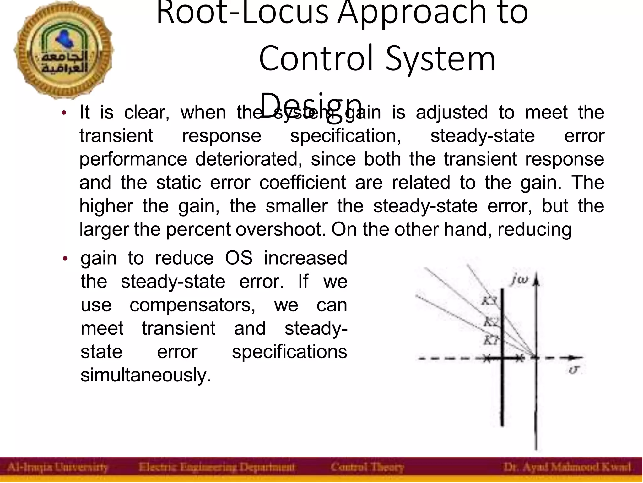
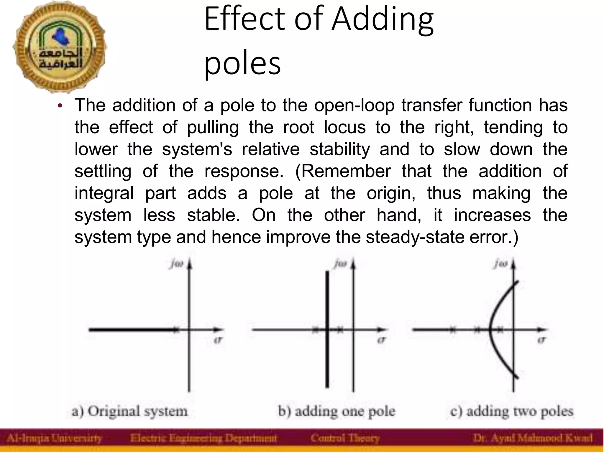
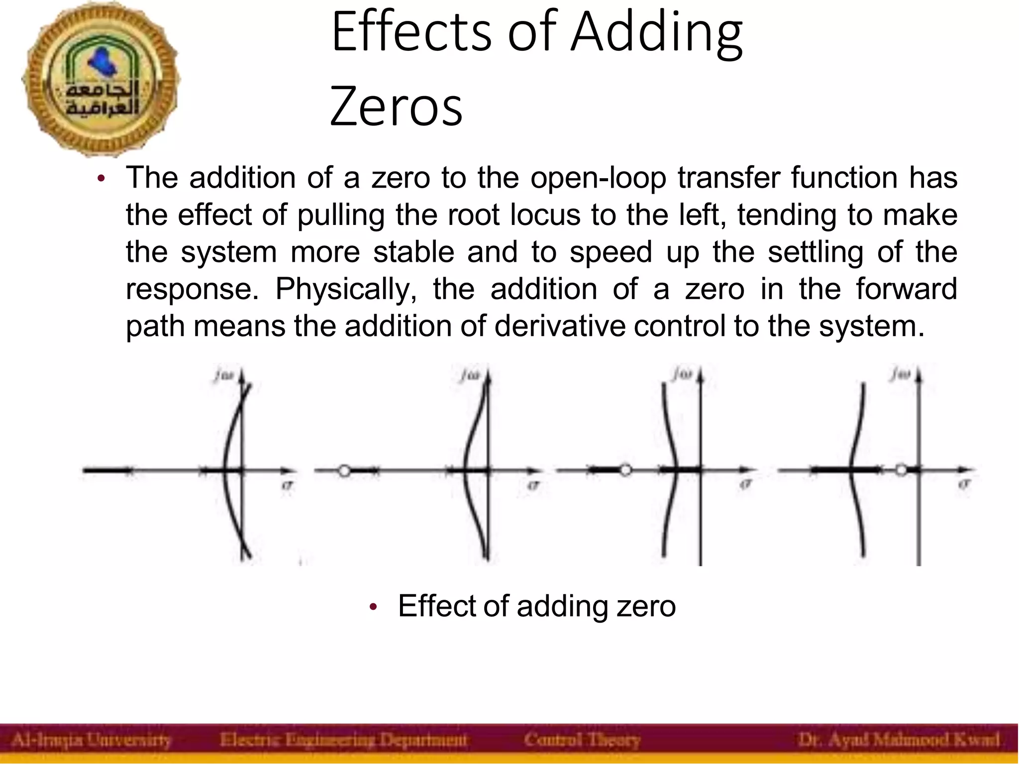
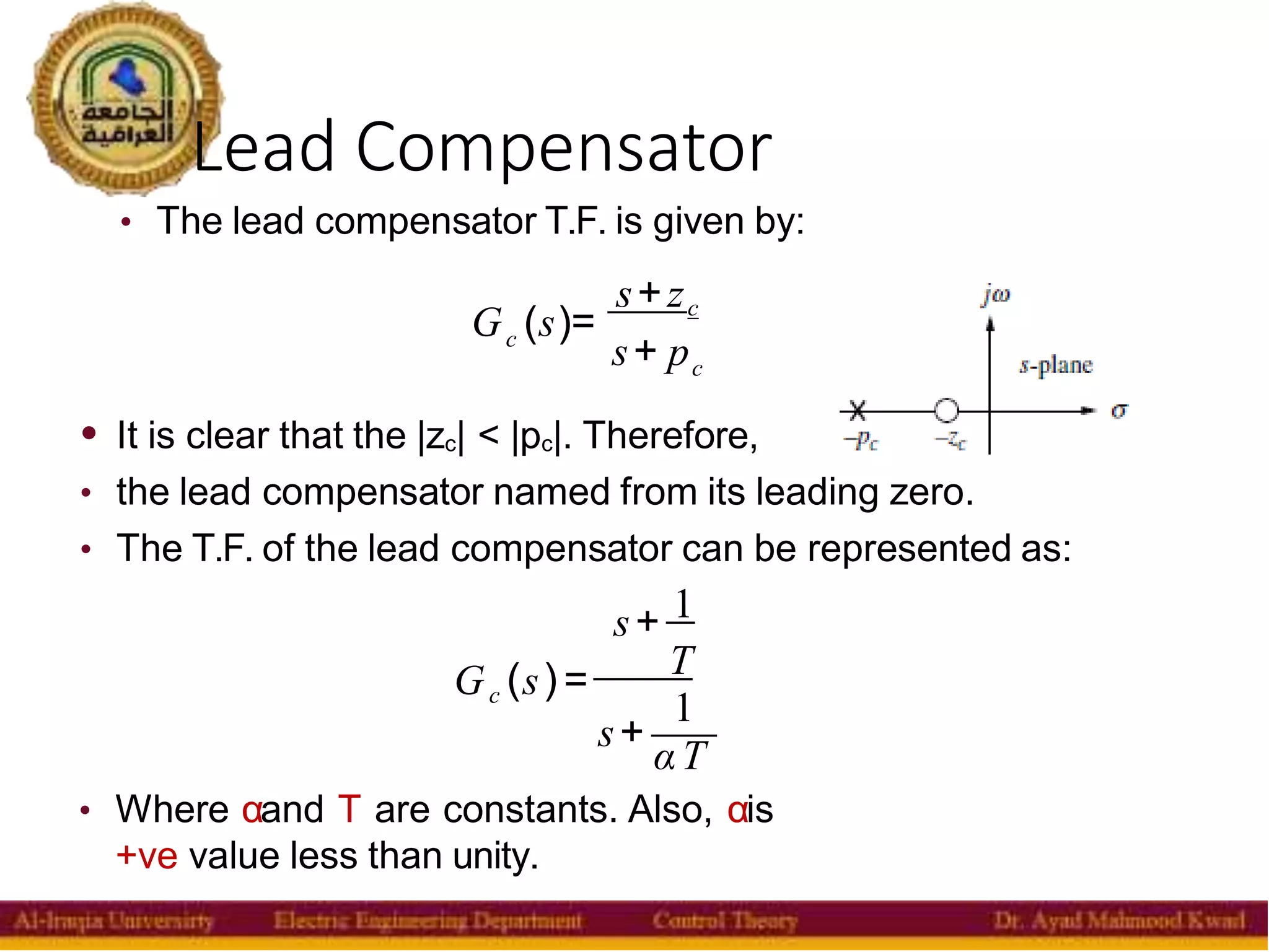
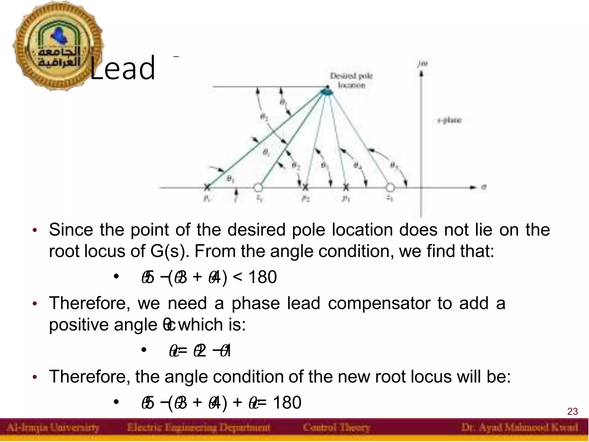
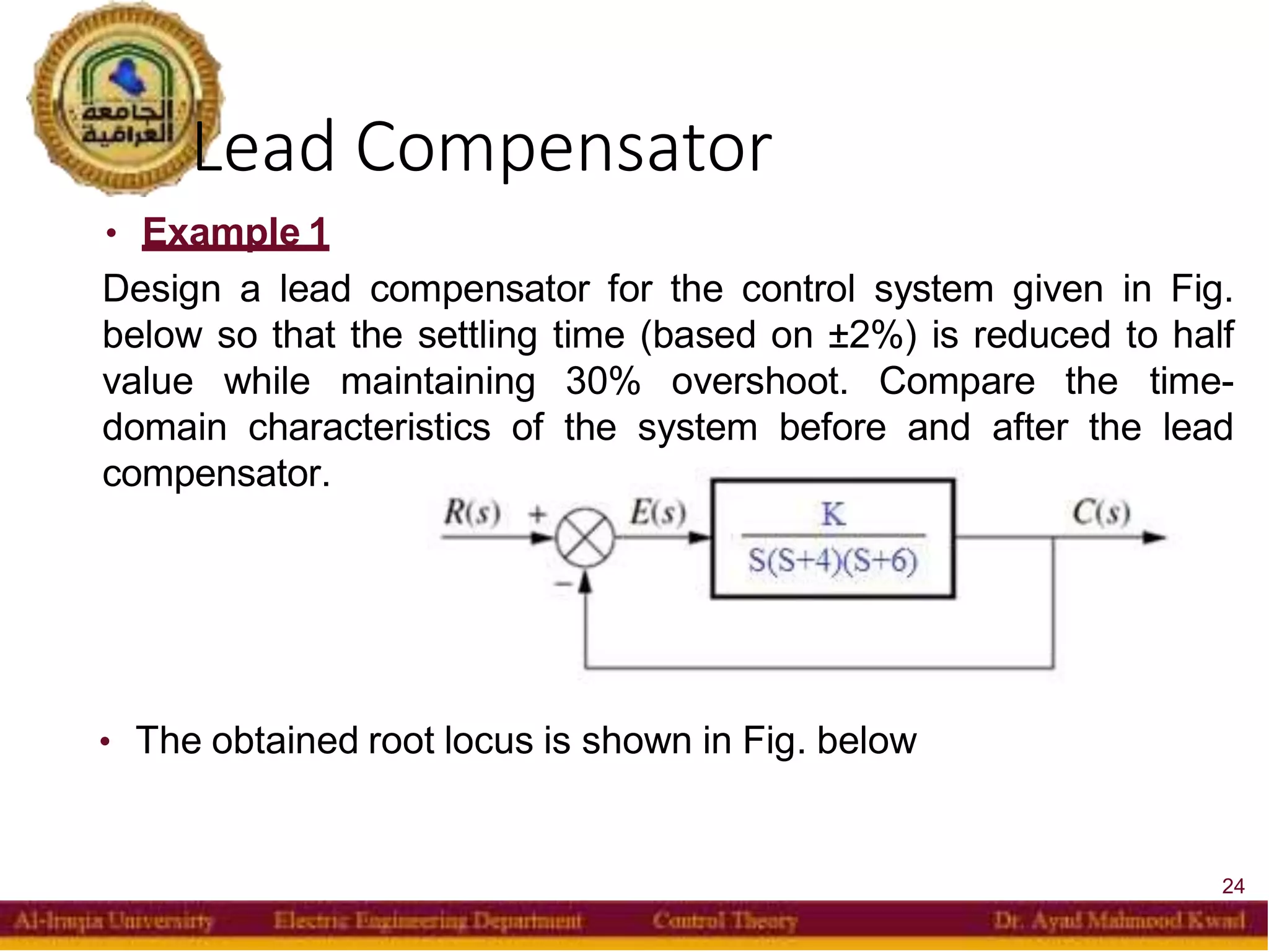
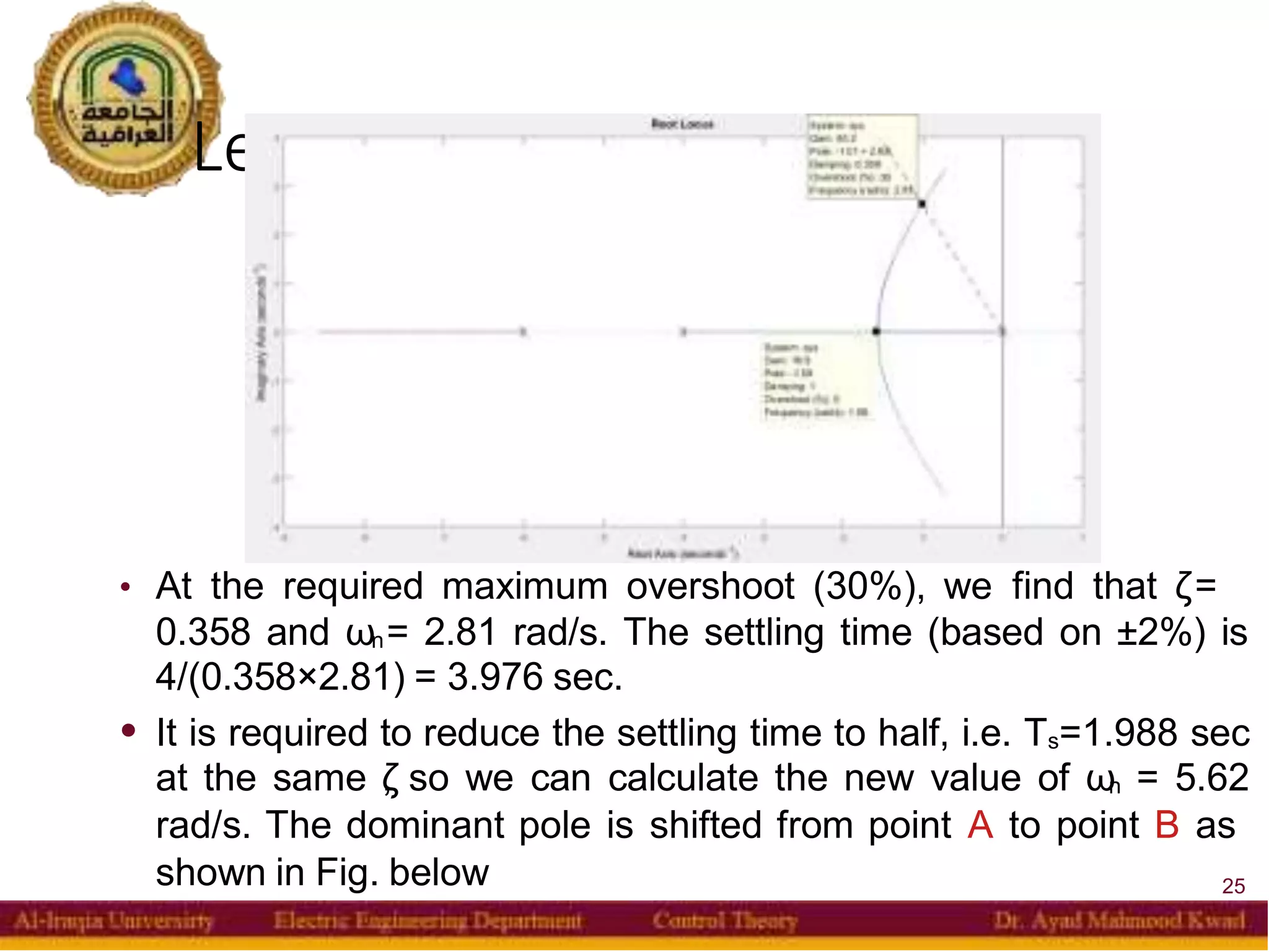
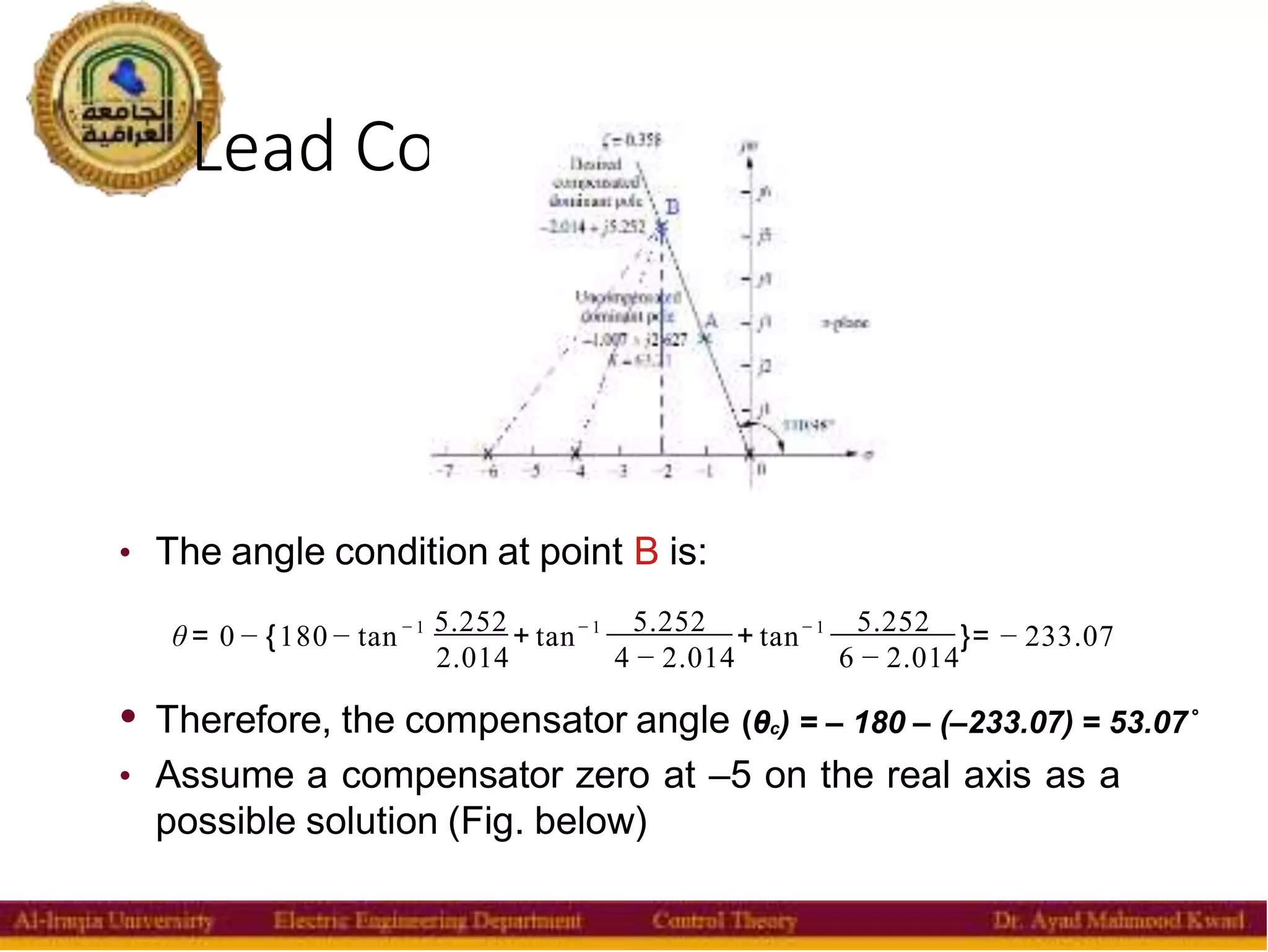
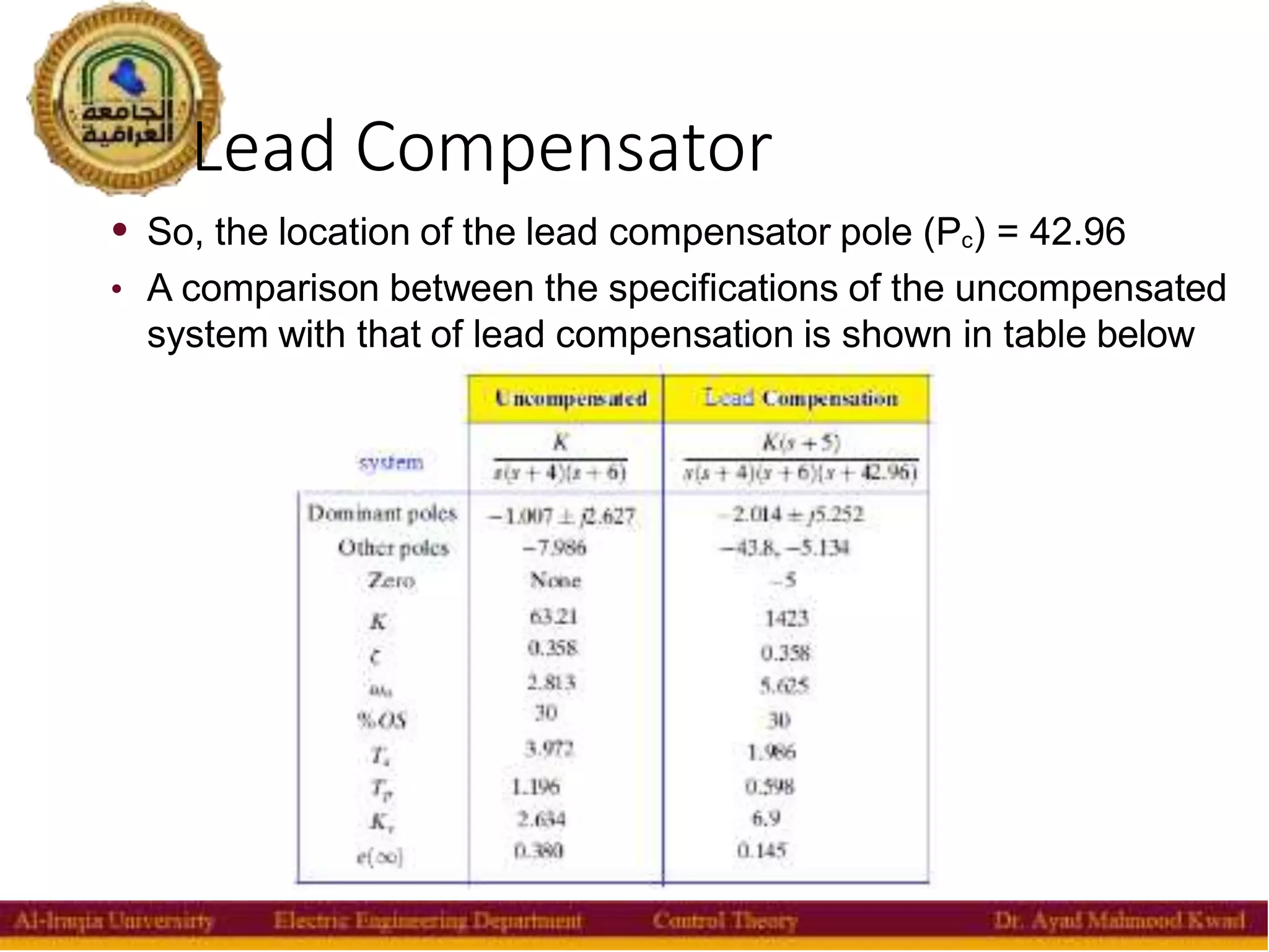
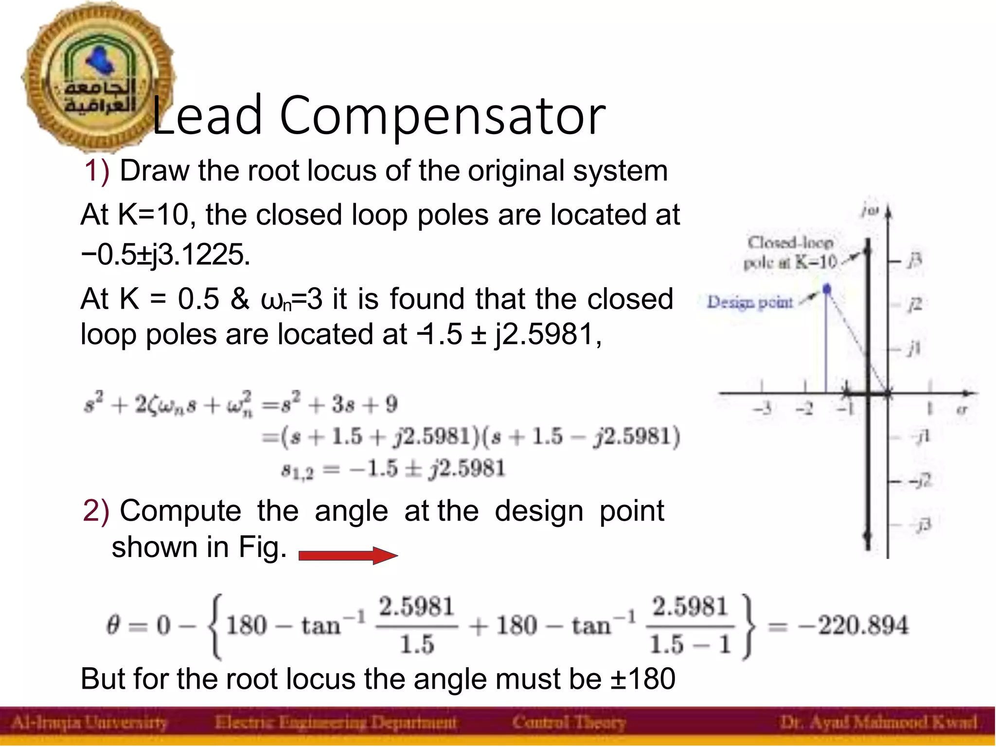
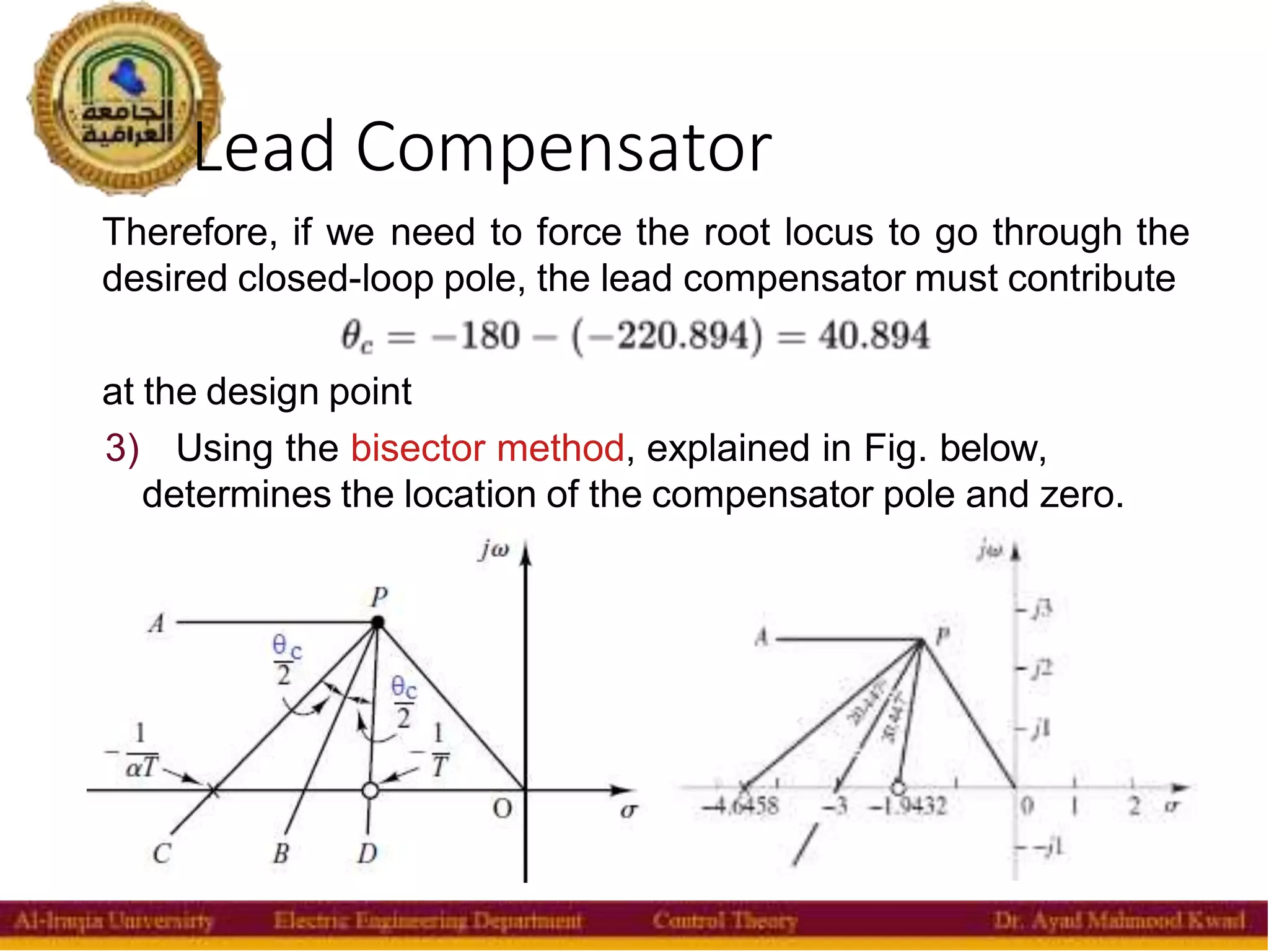
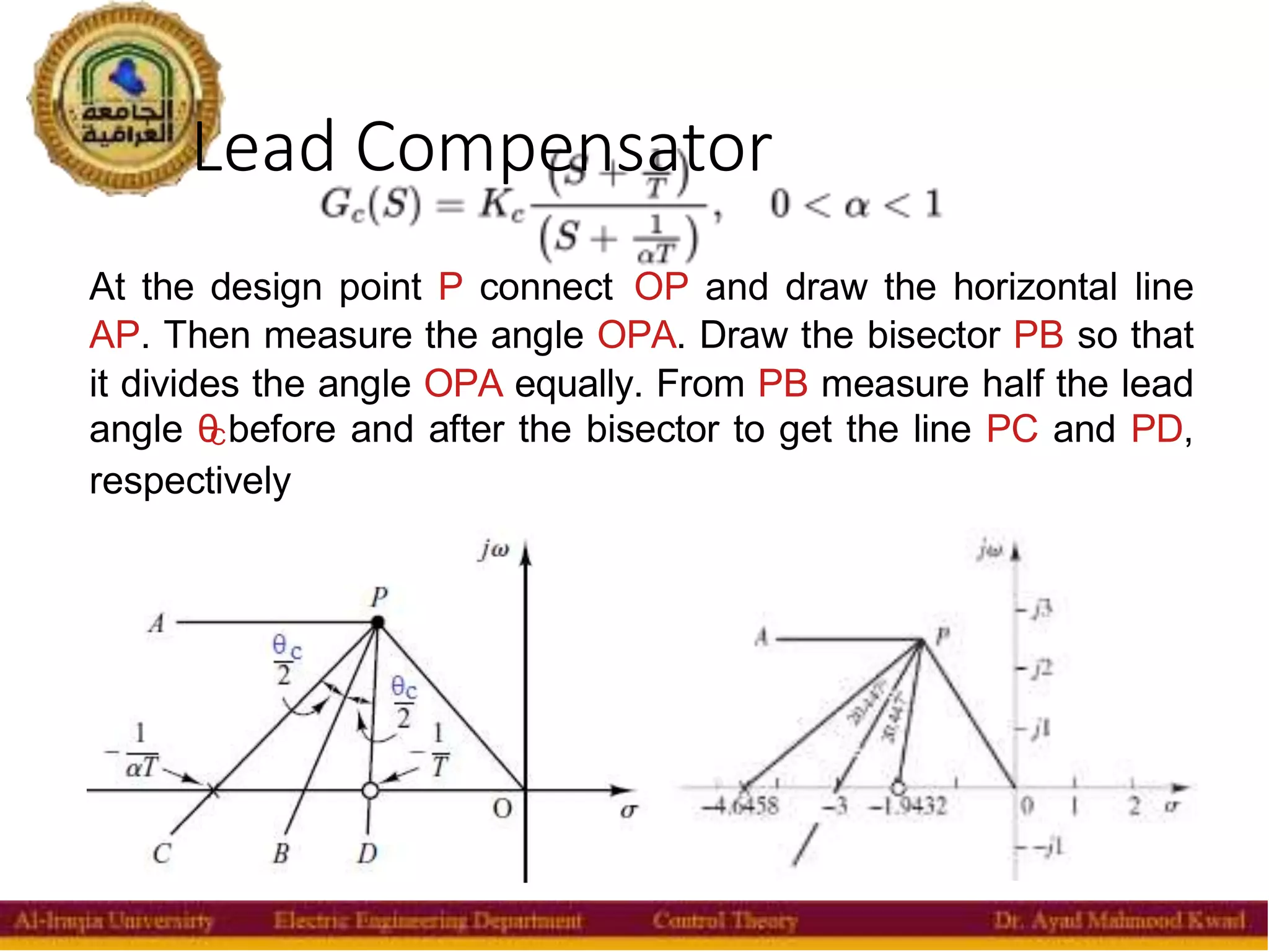
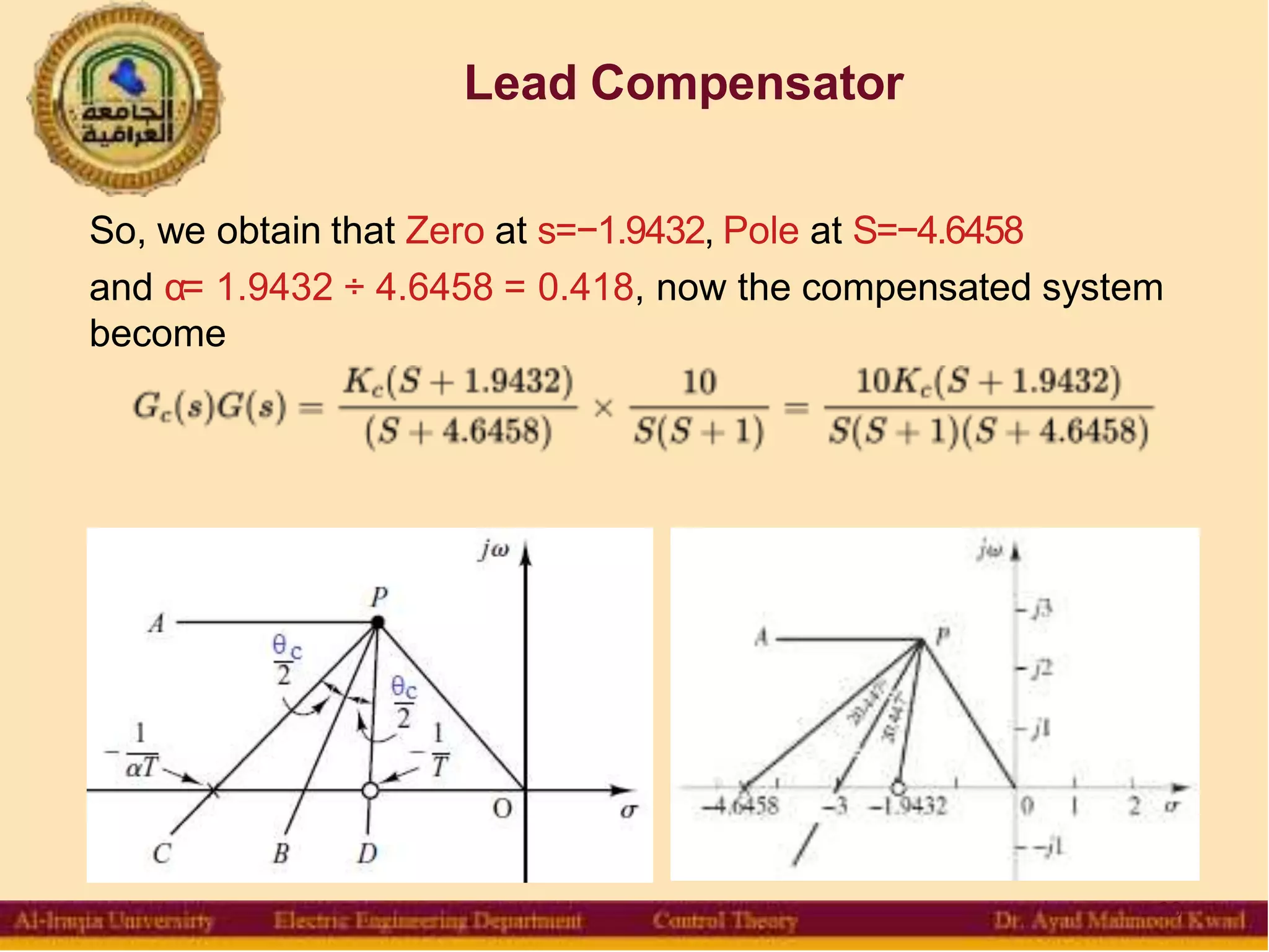
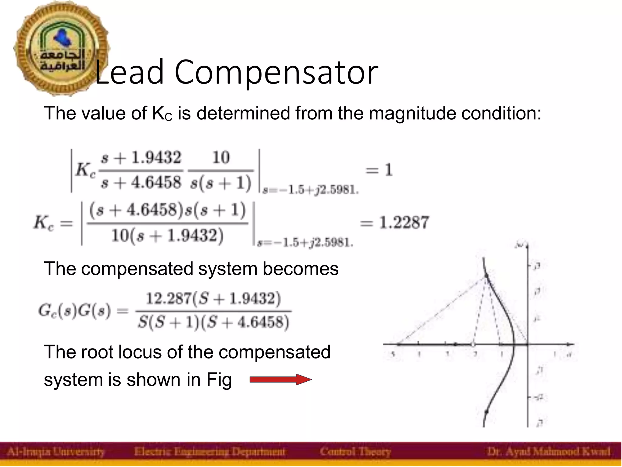
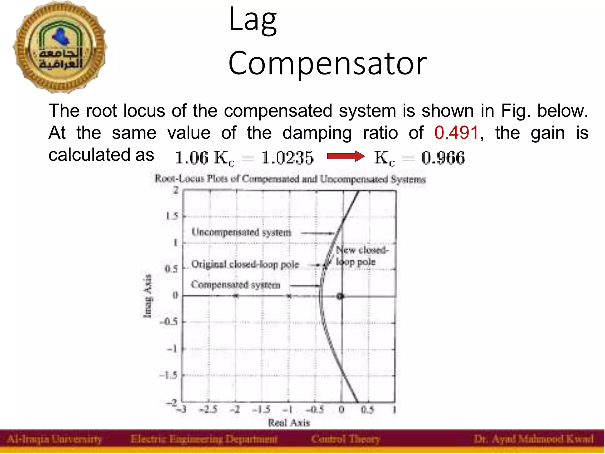
The document discusses control system design using root locus and PID tuning. It introduces root locus analysis and how adjusting the system gain can affect transient and steady-state response. PID controllers are commonly used compensators that can improve performance. The effects of proportional, integral and derivative controllers on closed-loop systems are described. An example mass-spring-damper system is analyzed with P, PI, PD and PID controllers to meet different performance specifications. Design procedures and effects of adding poles and zeros to the open-loop transfer function are also covered. Lead and lag compensators are discussed as ways to reshape the root locus to achieve desired closed-loop poles.

1. Chapter 6
Design by Root Locus and PID tuning
Control Engineering II : EE 4203
• AYAD MAHMOOD
• http://ayadmk.blogspot.com
/
• March 2, 2023
1

2. Introduct
ion
2
• Control systems are designed to perform specific tasks that
generally called performance specifications. These
specifications may be given in terms of transient response
(such as the maximum overshoot and settling time in step
response) and/or of steady-state requirements (such as
steady-state error).
• As the gain (K) is varied, both the transient and steady-state
responses are also varied. Setting K at a particular value
produces the transient response obtained by the poles at
• that point on the root locus. Thus, by changing K, we are
limited to those responses that exist along the root locus.

3. Introduct
ion
3
• For example, at a certain ( % OS, and settling time) is
desired, the transient response is represented by point B
shown in Fig. Below.
• At the specified % OS, we only can obtain the settling time
represented by point A with the suitable gain adjustment.
Thus, our goal is to speed up the response at A to that at
point B. This cannot be accomplished by a simple gain
adjustment, since point B does not lie on the root locus.

4. Introduct
ion
4
• The design by the root-locus method is based on reshaping
the root locus of the system by adding poles and zeros to
the system's open-loop transfer function and forcing the root
locus to pass through desired closed-loop poles in the s
plane.
• Adding pole or zero is done by a controller or compensator.
The additional poles and zeros can be generated with a
passive or an active network.
• Therefore, the compensator is a device inserted into the
system for the purpose of satisfying the specifications. The
compensator compensates for deficit performance of the
original system.

5. PID
Controller
5
• The compensator compensates for deficit performance of
the original system. Commonly used compensators or
controllers are:
• Lead compensator (PD controller)
• Lag compensator (PI controller)
• Lag-Lead compensator (PID controller)

6. • The transfer function of the PID controller looks like the
following:
• Kp = Proportional gain
• KI = Integral gain
• KD = Derivative gain
PID
Controller
6
C p D
G (s)= k +k s+
k I
s

7. Characteristics of P, I, and D
controllers
7
• A proportional controller (Kp) will have the effect of reducing
the rise time and will reduce, but never eliminate, the steady-
state error.
• An integral control (Ki) will have the effect of eliminating the
steady-state error, but it may make the transient response
worse.
• A derivative control (Kd) will have the effect of increasing the
stability of the system, reducing the overshoot, and
improving the transient response.
• Effects of each of controllers Kp, Kd, and Ki on a closed-
loop system are summarized in the table shown below.

8. Characteristics of P, I, and D controllers
RISE TIME OVERSHO
OT
SETTLING
TIME
Steady-State
Response
Kp Decrease Increase Small Change Decrease
Ki Decrease Increase Increase Eliminate
Kd Small
Change
Decrease Decrease Small Change
8

9. Example
Problem
9
and damper
• Suppose we have a simple mass, spring,
problem.
• The modeling equation of this system is
f (t )= M
d 2
x (t ) dx (t )
dt dt
+ f v +Kx (t )
X (s) 1
F (s)
=
s2
+10 s+20
• Let
• M = 1kg
• fv = 10 N.s/m
• k = 20 N/m
• F(s) = 1 = unit step

10. Open-loop step
response
10
• Let's first view the open-loop step
response.
• The DC gain of the plant transfer
function is 1/20, so 0.05 is the final value
of the output to an unit step input. This
corresponds to the steady-state error
of 0.95, quite large indeed.
• Furthermore, the rise time is about one
second, and the settling time is about 1.5
seconds.
• Let's design a controller that will reduce
the rise time, reduce the settling time,
and eliminates the steady-state error.

11. Closed Loop with P-
Controller
11
• The closed-loop T.F is
C (s)
R (s)
=
k p
2
s +10 s+ 20+k p
( )
• Let the proportional gain (Kp) equals
300.
• The plot shows that the
proportional controller reduced
both the rise time and the
steady-state error, increased the
overshoot, and decreased the
settling time by small amount.

12. Closed Loop with PD-
Controller
12
• The closed-loop T.F is
C (s) k p+ k D s
R (s)
=
s2
+(10+k )s+(20+ k )
D p
• Let Kp equals 300 and KD equals 10.
• The plot shows that the derivative
controller reduced both the
overshoot and the settling time, and
had small effect on the rise time and
the steady- state error.

13. Closed Loop with PI-
Controller
13
• The closed-loop T.F is
C (s)
R (s)
=
k p s+k I
3 2
( )
s +10 s + 20+k s+ k
p I
• Let Kp equals 30 and KI equals 70.
• We have reduced the (Kp) because
the integral controller also reduces
the rise time and increases the
overshoot as the proportional
controller does (double effect). The
above response shows that the
integral controller eliminated the
steady-state error.

14. Closed Loop with PID-
Controller
14
• The closed-loop T.F is
C (s ) k s2
+k s+ k
= D p I
R (s) s3
+(10+k )s2
+(20+k )s+k
D p I
• Let Kp equals 350, KD equals 50 and
KI equals 300.
• Now, we have obtained the system
with no overshoot, fast rise time,
and no steady- state error.

15. General tips for
designing a PID
controller
15
• When you are designing a PID controller for a given system,
follow the steps shown below to obtain a desired response.
1.Obtain an open-loop response and determine what
needs to be improved
2.Add a proportional control to improve the rise time
3.Add a derivative control to improve the overshoot
4.Add an integral control to eliminate the steady-state error
5.Adjust each of Kp, KI, and KD until you obtain a desired
overall response.

16. Realization of
Compensators
16
• The T.F. of the compensator is GC(s) and may be connected
in series as shown in (Fig. a) and is called series
compensator. Also, it can be connected in feedback as
shown in (Fig. b) and is called feedback compensator.
(a) (b)

17. Root-Locus Approach to
Control System
Design
17
• The root-locus method is a graphical method for determining
the locations of all closedloop poles based on the locations
of the open-loop poles and zeros as the gain K is varied
from zero to infinity (0-∞). As an example, consider the
system represented by
G (s) H (s )=
K
(s +1)(s+ 2)
• As shown from the system root
locus shown in Fig.→, as the gain
increases from K1 to K2 to K3 the
damping ratio decreases affecting
the transient performance but the
steady-state error is improved

18. Root-Locus Approach to
Control System
Design
18
• It is clear, when the system gain is adjusted to meet the
transient response specification, steady-state error
performance deteriorated, since both the transient response
and the static error coefficient are related to the gain. The
higher the gain, the smaller the steady-state error, but the
larger the percent overshoot. On the other hand, reducing
• gain to reduce OS increased
the steady-state error. If we
use compensators, we can
meet transient and steady-
state error specifications
simultaneously.

19. Effect of Adding
poles
19
• The addition of a pole to the open-loop transfer function has
the effect of pulling the root locus to the right, tending to
lower the system's relative stability and to slow down the
settling of the response. (Remember that the addition of
integral part adds a pole at the origin, thus making the
system less stable. On the other hand, it increases the
system type and hence improve the steady-state error.)

20. Effects of Adding
Zeros
20
• The addition of a zero to the open-loop transfer function has
the effect of pulling the root locus to the left, tending to make
the system more stable and to speed up the settling of the
response. Physically, the addition of a zero in the forward
path means the addition of derivative control to the system.
• Effect of adding zero

21. Lead Compensator
21
• The lead compensator T.F. is given by:
c
G (s)=
s+zc
s+ pc
c
• It is clear that the |zc| < |pc|. Therefore,
• the lead compensator named from its leading zero.
• The T.F. of the lead compensator can be represented as:
s+ 1
G (s)= T
1
s+
αT
• Where αand T are constants. Also, αis
+ve value less than unity.

22. Lead Compensator
22
• The procedure for designing a lead compensator for any
control system is:
3.
1. From the desired performance specifications, determine the
desired location for the dominant closed-loop poles.
2. By drawing the root-locus of the uncompensated (original) system
G(s), be sure that the gain adjustment alone can yield the desired
closed-loop poles. If not, calculate the angle deficiency θC. This
angle must be contributed by the lead compensator to reshape
the new root locus is to pass through the desired locations
obtained from step #1.
Determine the value of α and T from the deficiency angle (θC). To
explain the above steps, consider the control system G(s) with
two poles (P1 & P2) and one zero (Z1) as given in Fig. below.

23. Lead Compensator
23
• Since the point of the desired pole location does not lie on the
root locus of G(s). From the angle condition, we find that:
 𝜃
5 −(𝜃
3 + 𝜃
4) < 180
• Therefore, we need a phase lead compensator to add a
positive angle θ
cwhich is:
 𝜃
𝑐= 𝜃
2 −𝜃
1
• Therefore, the angle condition of the new root locus will be:
 𝜃
5 −(𝜃
3 + 𝜃
4) + 𝜃
𝑐= 180

24. Lead Compensator
24
• Example 1
Design a lead compensator for the control system given in Fig.
below so that the settling time (based on ±2%) is reduced to half
value while maintaining 30% overshoot. Compare the time-
domain characteristics of the system before and after the lead
compensator.
• The obtained root locus is shown in Fig. below

25. Lead Compensator
25
• At the required maximum overshoot (30%), we find that ζ=
0.358 and ωn= 2.81 rad/s. The settling time (based on ±2%) is
4/(0.358×2.81) = 3.976 sec.
• It is required to reduce the settling time to half, i.e. Ts=1.988 sec
at the same ζ
, so we can calculate the new value of ωn = 5.62
rad/s. The dominant pole is shifted from point A to point B as
shown in Fig. below

26. Lead Compensator
26
• The angle condition at point B is:
θ = 0 − {180− tan− 1 5.252 + tan− 1 5.252 + tan− 1 5.252 }= − 233.07
2.014 4 − 2.014 6 − 2.014
• Therefore, the compensator angle (θc) = – 180 – (–233.07) = 53.07˚
• Assume a compensator zero at –5 on the real axis as a
possible solution (Fig. below)

27. Lead Compensator
27
zc
5 − 2.014
θ =tan− 1 5.252 =60.38
θ pc = θ zc − θc = 60.38− 53.07= 7.31
pc
tan θ =0.1283= 5.252
c
P − 2.014 c
P =42.96

28. Lead Compensator
28
• So, the location of the lead compensator pole (Pc) = 42.96
• A comparison between the specifications of the uncompensated
system with that of lead compensation is shown in table below

29. Lead Compensator
• s(s+1)
• It is desired to make the system damping ratio 0.5 with
undamped natural frequency 3.0 rad/s. Design the suitable lead
compensator and draw the root locus of the compensated
system
29
• Example 2
Consider the unity feedback control system:
G(s)= 10

30. Lead Compensator
30
1) Draw the root locus of the original system
At K=10, the closed loop poles are located at
−0.5±j3.1225.
At K = 0.5 & ωn=3 it is found that the closed
loop poles are located at −
1.5 ± j2.5981,
2) Compute the angle at the design point
shown in Fig.
But for the root locus the angle must be ±180

31. Lead Compensator
31
Therefore, if we need to force the root locus to go through the
desired closed-loop pole, the lead compensator must contribute
at the design point
3) Using the bisector method, explained in Fig. below,
determines the location of the compensator pole and zero.

32. Lead Compensator
32
At the design point P connect OP and draw the horizontal line
AP. Then measure the angle OPA. Draw the bisector PB so that
it divides the angle OPA equally. From PB measure half the lead
angle θ
Cbefore and after the bisector to get the line PC and PD,
respectively

33. Lead Compensator
So, we obtain that Zero at s=−1.9432, Pole at S=−4.6458
and α= 1.9432 ÷ 4.6458 = 0.418, now the compensated system
become
33

34. Lead Compensator
34
The value of KC is determined from the magnitude condition:
The compensated system becomes
The root locus of the compensated
system is shown in Fig

35. Lag
Compensator
35
The lag compensator T.F. is given by
Where β > 1.


The lag compensator used when the system exhibits fine
transient-response characteristics but unsatisfactory steady-
state characteristics.
Compensation in this case basically consists of increasing
the open-loop gain without appreciably changing the
transient-response characteristics. This means that the root
locus in the vicinity of the dominant closed-loop poles should
not be changed appreciably, but the open-loop gain should
be increased as much as needed

36. Lag
Compensator
36


To avoid an appreciable change in the root locus, the angle
contribution of the lag network should be limited to a small
amount, say 5° or less. To assure this, we place the pole
and zero of the lag network relatively close together and
near the origin of the s-plane. Then the closed-loop poles of
the compensated system will be shifted only slightly from
their original locations. Hence, the transient-response
characteristics will be changed only slightly.
If we place the zero and pole of the lag compensator very
close to each other, that means:
and

37. Lag
Compensator
37
• Example 3
Consider the unity feedback control system:
At a damping ratio of 0.491, it is required to make the velocity
error coefficient = 5, Design the suitable lag compensator & draw
the root locus of the compensated system.
From the root locus of the
uncompensated system, the
closed loop poles at = 0.491 are
located at s = -0.3307 ± j 0.5864
as shown in Fig

38. Lag
Compensator
38
From the magnitude condition, K = 1.06, the static velocity error
coefficient Kv = 1.06 / 2 = 0.53, the required velocity error
coefficient Kv is 5, this mean
So,
Let T = 2β= 2 × 9.434 = 18.868, therefore, the lag zero is located
at 1/T = 0.053, and the lag pole is located at 1/βT = 0.0056. The
compensated system is

39. Lag
Compensator
39
The root locus of the compensated system is shown in Fig. below.
At the same value of the damping ratio of 0.491, the gain is
calculated as

40. Referen
ces
40
1. Norman S. Nise, Control Systems Engineering (6th Edition), John
2. Wiley and Sons, 2011.
3. Katsuhiko Ogata, Modern Control Engineering (5th Edition),
4. Pearson Education International, Inc., 2010.
5. Richard C. Dorf and Robert H. Bishop, Modern Control Systems (12th Edition), Pearson
Educational International, 2011.
6. Rao V. Dukkipati, Analysis and Design of Control systems Using MATLAB, Published
by New Age International (P) Ltd., Publishers, 2006.
7. Katsuhiko Ogata, MATLAB For Control Engineers, Pearson Education International,
Inc., 2008.