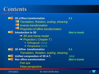
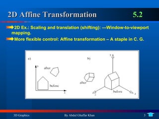
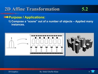
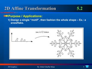
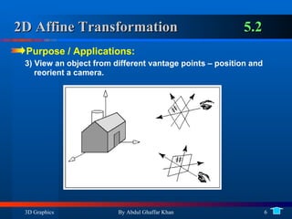
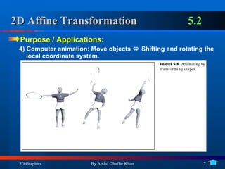
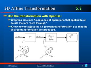
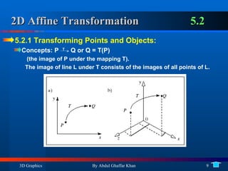
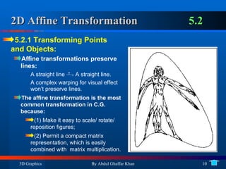
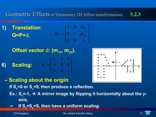
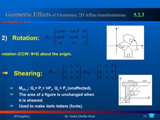
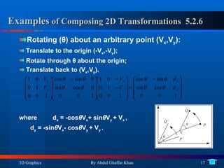
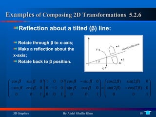
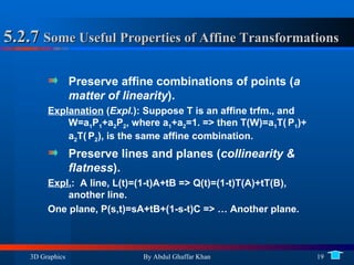
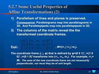
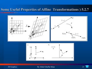
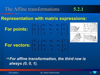
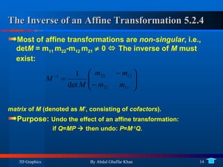
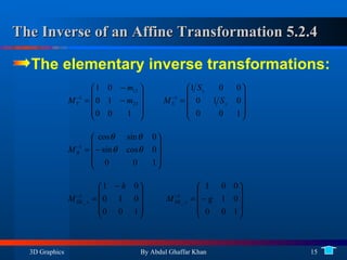
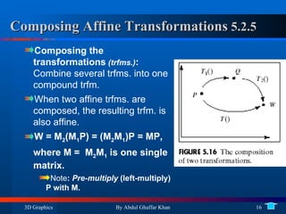
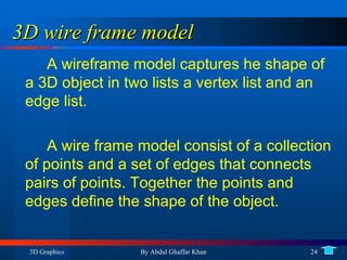
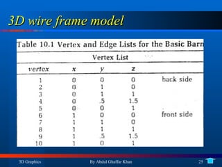
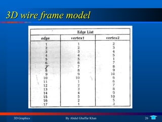
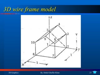
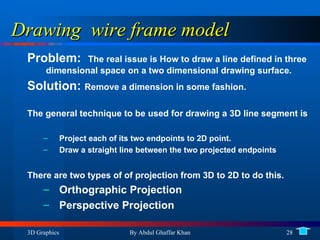
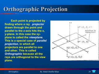
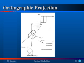
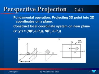
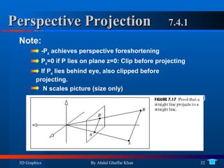
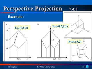
This document provides an overview of 2D and 3D graphics transformations including: 1. 2D affine transformations like translation, rotation, scaling and shearing and their properties such as preserving lines and ratios. 2. Representing transformations with matrices and composing multiple transformations. 3. Drawing 3D wireframe models using projections including orthogonal and perspective projections. 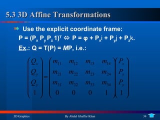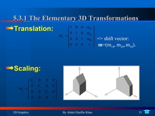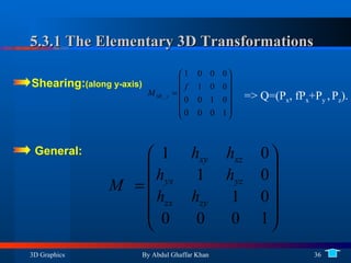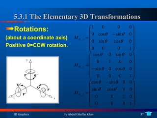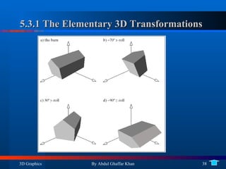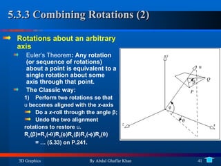4. 3D affine transformations and their elementary forms as well as composing rotations in 3D. 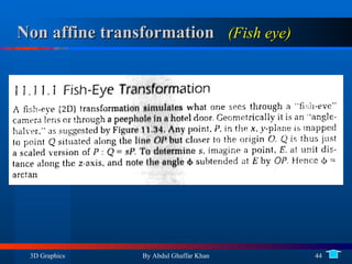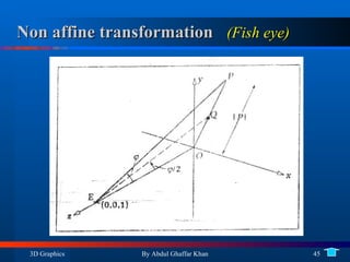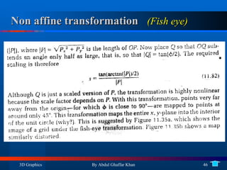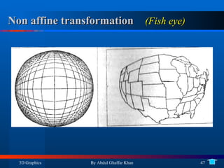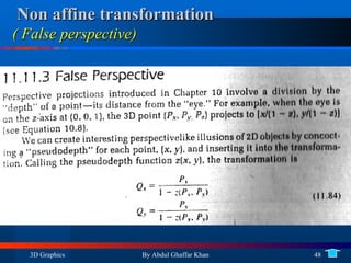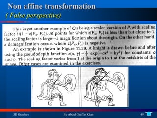5. Non-affine transformations like fish-eye and false perspective distortions.

1. 3D Graphics A Lecture By Abdul Ghaffar

2. Contents 2D a1ffine transformation 5.2 Translation, Rotation, scaling, shearing Inverse transformation Properties of affine transformation Introduction to 3D (Not in book) 3D wire frame model Projection ( Chapter 7 ) Orthogonal (7.6.2) Perspective (7.4.1) 3D Affine transformation 5.3 Translation, Rotation, scaling, shearing Unified composition of 3D A.T. 5.3.2 Non affine transformation (Not in book) Fish eye False perspective

3. 2D Affine Transformation 5.2 2D Ex.: Scaling and translation (shifting): —Window-to-viewport mapping. More flexible control: Affine transformation – A staple in C. G.

4. 2D Affine Transformation 5.2 Purpose / Applications: Compose a “scene” out of a number of objects – Applied many instances.

5. 2D Affine Transformation 5.2 Purpose / Applications: Design a single “motif”, then fashion the whole shape – Ex.: a snowflake.

6. 2D Affine Transformation 5.2 Purpose / Applications: 3) View an object from different vantage points – position and reorient a camera.

7. 2D Affine Transformation 5.2 Purpose / Applications: 4) Computer animation: Move objects  Shifting and rotating the local coordinate system.

8. 2D Affine Transformation 5.2 Use the transformation with OpenGL: Graphics pipeline: A sequence of operations that applied to all points that are “sent through”. Know how to adjust the CT (current transformation ) so that the desired transformation are produced.

9. 2D Affine Transformation 5.2 5.2.1 Transforming Points and Objects: Concepts: P T > Q or Q = T(P) (the image of P under the mapping T). The image of line L under T consists of the images of all points of L.

10. 2D Affine Transformation 5.2 5.2.1 Transforming Points and Objects: Affine transformations preserve lines: A straight line T > A straight line. A complex warping for visual effect won’t preserve lines. The affine transformation is the most common transformation in C.G. because: (1) Make it easy to scale/ rotate/ reposition figures; (2) Permit a compact matrix representation, which is easily combined with matrix multiplication.

11. The Affine transformations 5.2.1 Representation with matrix expressions: For points: For vectors: For affine transformation, the third row is always (0, 0, 1).

12. Geometric Effects of Elementary 2D Affine transformations 5.2.3 Translation: Q=P+ d , Offset vector d : (m 13 , m 23 ). Scaling: – Scaling about the origin. If S x <0 or S y <0, then produce a reflection. Ex.: S x =-1,  A mirror image by flipping it horizontally about the y-axis. If S x =S y =S, then have a uniform scaling.

13. Geometric Effects of Elementary 2D Affine transformations 5.2.3 Rotation: rotation (CCW: θ>0 ) about the origin . Shearing: M SR_x : Q x = P x + hP y , Q y = P y (unaffected). The area of a figure is unchanged when it is sheared. Used to make italic letters (fonts).

14. The Inverse of an Affine Transformation 5.2.4 Most of affine transformations are non-singular , i.e., det M = m 11 m 22 -m 12 m 21  0  The inverse of M must exist: matrix of M (denoted as M * , consisting of cofactors ). Purpose: Undo the effect of an affine transformation: if Q = MP  then undo: P = M -1 Q .

15. The Inverse of an Affine Transformation 5.2.4 The elementary inverse transformations:

16. Composing Affine Transformations 5.2.5 Composing the transformations (trfms.) : Combine several trfms. into one compound trfm. When two affine trfms. are composed, the resulting trfm. is also affine. W = M 2 (M 1 P) = (M 2 M 1 )P = MP, where M = M 2 M 1 is one single matrix. Note : Pre-multiply (left-multiply) P with M.

17. Examples of Composing 2D Transformations 5.2.6 Rotating ( θ) about an arbitrary point (V x ,V y ): Translate to the origin (-V x ,-V y ); Rotate through θ about the origin; Translate back to (V x ,V y ). where d x = -cos θ V x + sin θ V y + V x , d y = -sin θ V x - cos θ V y + V y .

18. Examples of Composing 2D Transformations 5.2.6 Reflection about a tilted ( β ) line: Rotate through β to x-axis; Make a reflection about the x-axis; Rotate back to β position.

19. 5.2.7 Some Useful Properties of Affine Transformations Preserve affine combinations of points ( a matter of linearity ). Explanation ( Expl. ): Suppose T is an affine trfm., and W=a 1 P 1 +a 2 P 2 , where a 1 +a 2 =1. => then T(W)=a 1 T( P 1 )+ a 2 T( P 2 ), is the same affine combination. Preserve lines and planes ( collinearity & flatness ). Expl. : A line, L(t)=(1-t)A+tB => Q(t)=(1-t)T(A)+tT(B), another line. One plane, P(s,t)=sA+tB+(1-s-t)C => … Another plane.

20. 5.2.7 Some Useful Properties of Affine Transformations (2) Parallelism of lines and planes is preserved. Consequence : Parallelograms map into parallelograms in 2D. And Parallelepipeds map into parallelepipeds in 3D. The columns of the matrix reveal the the transformed coordinate frames. Expl. : , M =( m 1 | m 2 | m 3 ). The coordinate frame ( i , j , φ ) that is defined by φ=(0 0 1) T , i =(1 0 0) T , j =(0 1 0) T transforms into ( m 1 , m 2 , m 3 ). For example, m 1 = M i . The axes of the new coordinate frame are not necessarily perpendicular, nor must they be of unit length .

21. Some Useful Properties of Affine Transformations ) 5.2.7

22. 5.2.7 Some Useful Properties of Affine Transformations (4) Relative ratios are preserved. Consequence : (a) Midpoints of lines map into midpoints. (b) The diagonals of any parallelogram bisect each other (because any parallelogram is an affine transformed square). (c) Preserve ellipses and ellipsoids, too. Effect of transformations on the areas of figures. Expl. : In 2D, (Area after trfm.)/(Area before trfm.) = |det M |. In 3D, similar arguments apply (to the volume of an object).

23. 5.2.7 Some Useful Properties of Affine Transformations (5) Every affine transformation is composed of elementary operations. Expl .: A matrix M can be factored into a product of elementary matrices in various ways. (a) For 2D decomposition ( from right to left ): M = (translation)(shear)(scaling)(rotation); (b) For 3D decomposition : M = (translation)(scaling)(rotation)(shear1)(shear2). Self study : All examples and exercises

24. 3D wire frame model A wireframe model captures he shape of a 3D object in two lists a vertex list and an edge list. A wire frame model consist of a collection of points and a set of edges that connects pairs of points. Together the points and edges define the shape of the object.

25. 3D wire frame model

26. 3D wire frame model

27. 3D wire frame model

28. Drawing wire frame model Problem: The real issue is How to draw a line defined in three dimensional space on a two dimensional drawing surface. Solution: Remove a dimension in some fashion. The general technique to be used for drawing a 3D line segment is Project each of its two endpoints to 2D point. Draw a straight line between the two projected endpoints There are two types of of projection from 3D to 2D to do this. Orthographic Projection Perspective Projection

29. Orthographic Projection Each point is projected by finding where a ray , projector drawn through the point and parallel to the z-axis hits the x, y-plane. In this case the xy-plane is called the viewplane . This is a special case of parallel projection , in which all projectors are parallel to one and other. This is called Orthographic because all the rays are orthogonal to the view plane.

30. Orthographic Projection

31. Perspective Projection 7.4.1 Fundamental operation: Projecting 3D point into 2D coordinates on a plane. Construct local coordinate system on near plane (x*,y*) = (N(P x /(-P z )), N(P y ,/(-P z ))

32. Perspective Projection 7.4.1 Note: -P z achieves perspective foreshortening P z =0 if P lies on plane z=0: Clip before projecting If P z lies behind eye, also clipped before projecting. N scales picture (size only) Straight lines project to straight lines (proof given)

33. Perspective Projection 7.4.1 Example: Eye(0,0,2) Eye(0.5,0,2) Eye(2,5,2)

34. 5.3 3D Affine Transformations Use the explicit coordinate frame: P = (P x P y P z 1 ) T  P = φ + P x i + P y j + P z k . Ex .: Q = T(P) = M P, i.e.:

35. 5.3.1 The Elementary 3D Transformations Translation: Scaling: => shift vector: m =(m 14 , m 24 , m 34 ).

36. 5.3.1 The Elementary 3D Transformations Shearing: (along y-axis) General: => Q=(P x , fP x +P y , P z ).

37. 5.3.1 The Elementary 3D Transformations Rotations: (about a coordinate axis) Positive θ =CCW rotation.

38. 5.3.1 The Elementary 3D Transformations

39. 5.3.2 Composing 3D Affine Transformations Similar to the 2D case, M = M 2 M 1 . Any number of affine transformations can be composed in this way.

40. 5.3.3 Combining Rotations One important distinction between 2D and 3D trfms. is the rotations combination . In 2D, R( β 1 ) and R( β 2 ) combine to produce R( β 1 + β 2 ). And the order makes no difference. In 3D, the order does matter: 3D rotation matrices do not commute. Any 3D rotation can be obtained by three rolls about the x-, y-, and z-axes: the overall rotation M = R z ( β 3 )R y ( β 2 )R x ( β 1 ), where β 1 , β 2 , and β 3 are called Euler angles . It takes three values to completely specify a rotation. There are 12 possible orderings of the three individual rolls, and each uses different values for β 1 , β 2 , and β 3 .

41. 5.3.3 Combining Rotations (2) Rotations about an arbitrary axis Euler’s Theorem : Any rotation (or sequence of rotations) about a point is equivalent to a single rotation about some axis through that point. The Classic way: Perform two rotations so that u becomes aligned with the x -axis Do a x -roll through the angle β ; Undo the two alignment rotations to restore u . R u ( β )=R y (-  )R z (  )R x ( β )R z (-  )R y (  ) = … (5.33) on P.241.

42. 5.3.4 Properties of 3D Affine Transformations Note : Stated in terms of any 3D trfms. T (.) or M . Preserve affine combinations of points. Preserve lines and planes. Parallelism of lines and planes is preserved. The columns of the matrix reveal the the transformed coordinate frames. Relative ratios are preserved. Effect of trfms. on the volumes of figures. Every affine transformation is composed of elementary operations.

43. Non affine transformation (Fish eye)

44. Non affine transformation (Fish eye)

45. Non affine transformation (Fish eye)

46. Non affine transformation (Fish eye)

47. Non affine transformation (Fish eye)

48. Non affine transformation ( False perspective)

49. Non affine transformation ( False perspective)