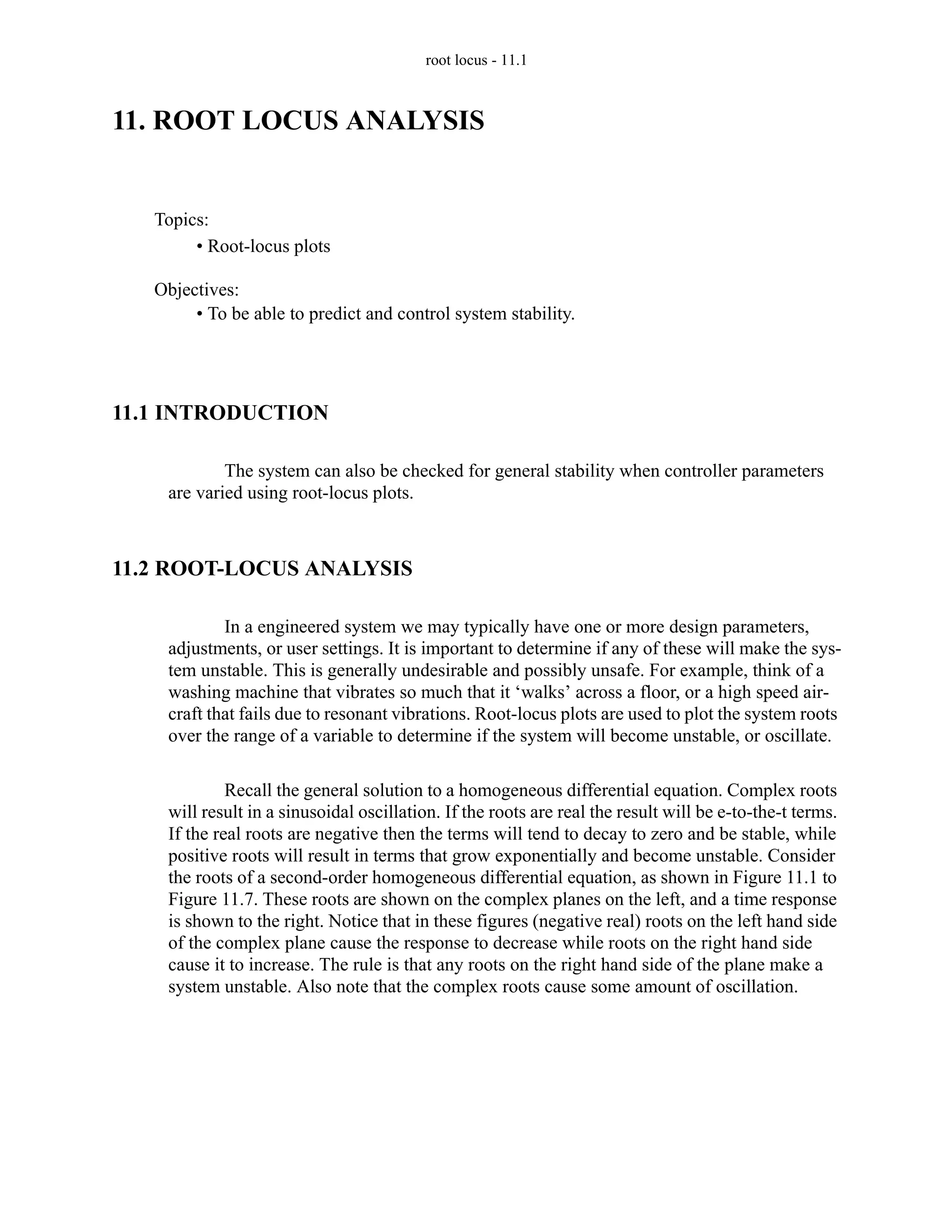
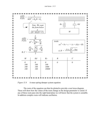
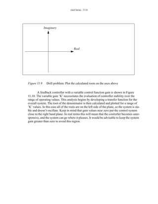
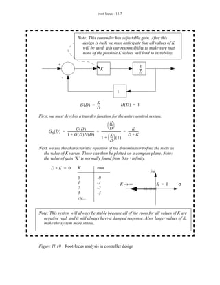
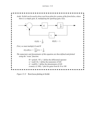
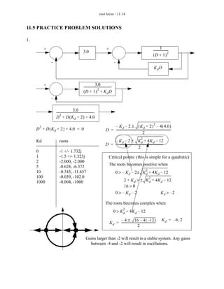
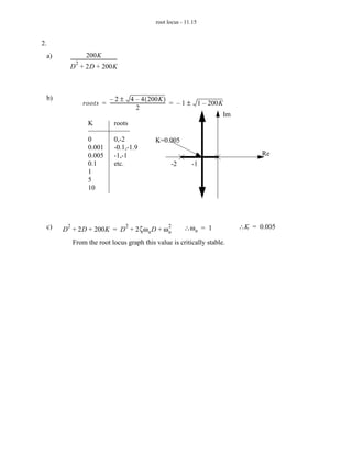
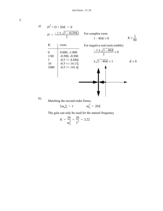
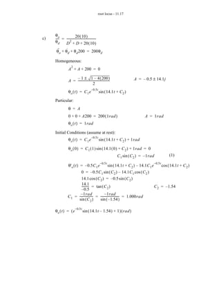
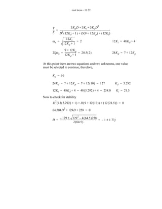
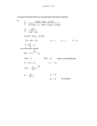
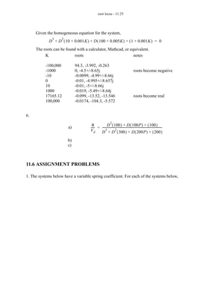
Root locus analysis

root locus - 11.1

11. ROOT LOCUS ANALYSIS

Topics:
• Root-locus plots

Objectives:
• To be able to predict and control system stability.

11.1 INTRODUCTION

The system can also be checked for general stability when controller parameters
are varied using root-locus plots.

11.2 ROOT-LOCUS ANALYSIS

In a engineered system we may typically have one or more design parameters,
adjustments, or user settings. It is important to determine if any of these will make the sys-
tem unstable. This is generally undesirable and possibly unsafe. For example, think of a
washing machine that vibrates so much that it ‘walks’ across a floor, or a high speed air-
craft that fails due to resonant vibrations. Root-locus plots are used to plot the system roots
over the range of a variable to determine if the system will become unstable, or oscillate.

Recall the general solution to a homogeneous differential equation. Complex roots
will result in a sinusoidal oscillation. If the roots are real the result will be e-to-the-t terms.
If the real roots are negative then the terms will tend to decay to zero and be stable, while
positive roots will result in terms that grow exponentially and become unstable. Consider
the roots of a second-order homogeneous differential equation, as shown in Figure 11.1 to
Figure 11.7. These roots are shown on the complex planes on the left, and a time response
is shown to the right. Notice that in these figures (negative real) roots on the left hand side
of the complex plane cause the response to decrease while roots on the right hand side
cause it to increase. The rule is that any roots on the right hand side of the plane make a
system unstable. Also note that the complex roots cause some amount of oscillation.

root locus - 11.2

R = – A, – B
jw x(t)

x0
-A -B
sigma

t

Figure 11.1 Negative real roots make a system stable

R = ± Aj
jw x(t)
A

sigma
-A
t

Figure 11.2 Complex roots make a system oscillate

R = – A ± Bj
jw x(t)
B

-A
sigma

-B t

Figure 11.3 Negative real and complex roots cause decaying oscillation

root locus - 11.3

R = – A ± Bj
jw x(t)
B

-A
sigma

-B t

Figure 11.4 More negative real and complex roots cause a faster decaying oscillation

R = – A, – A
jw x(t)

-A,-A
sigma

t

Figure 11.5 Overlapped roots are possible

R = A, A
jw x(t)

A,A
sigma

t

Figure 11.6 Positive real roots cause exponential growth and are unstable

root locus - 11.4

R = A ± Bj
jw x(t)
B

A sigma

-B t

Figure 11.7 Complex roots with positive real parts have growing oscillations and are
unstable

Next, recall that the denominator of a transfer function is the homogeneous equa-
tion. By analyzing the function in the denominator of a transfer function the general sys-
tem response can be found. An example of root-locus analysis for a mass-spring-damper
system is given in Figure 11.8. In this example the transfer function is found and the roots
of the equation are written with the quadratic equation. At this point there are three
unspecified values that can be manipulated to change the roots. The mass and damper val-
ues are fixed, and the spring value will be varied. The range of values for the spring coef-
ficient should be determined by practical and design limitations. For example, the spring
coefficient should not be zero or negative.

root locus - 11.5

x( D) 1
------------ = -----------------------------------------
- -
F(D) 2
MD + K d D + K s

Note: We want Ks Kd
the form below
A
--------------------------------------
- M
(D + B)(D + C)
1-
----
x(D) M
------------ = ------------------------------------
- -
F(D) 2 Kd Ks Aside:
D + ----- D + -----
-
M M 2
ax + bx + c = ( x + A ) ( x + B )
2
–Kd Kd Ks
-------- ± ------ – 4 -----
- - – b ± b – 4ac
2
M M
2 M A, B = --------------------------------------
B, C = ------------------------------------------
- 2a
2

M Kd Ks B C

0 0 0 0 0
100 100 100
100 100 1000
100 100 10000

Figure 11.8 A mass-spring-damper system equation

The roots of the equation can then be plotted to provide a root locus diagram.
These will show how the values of the roots change as the design parameter is varied. If
any of these roots pass into the right hand plane we will know that the system is unstable.
In addition complex roots will indicate oscillation.

root locus - 11.6

Imaginary

Real

Figure 11.9 Drill problem: Plot the calculated roots on the axes above

A feedback controller with a variable control function gain is shown in Figure
11.10. The variable gain ’K’ necessitates the evaluation of controller stability over the
range of operating values. This analysis begins by developing a transfer function for the
overall system. The root of the denominator is then calculated and plotted for a range of
’K’ values. In this case all of the roots are on the left side of the plane, so the system is sta-
ble and doesn’t oscillate. Keep in mind that gain values near zero put the control system
close to the right hand plane. In real terms this will mean that the controller becomes unre-
sponsive, and the system can go where it pleases. It would be advisable to keep the system
gain greater than zero to avoid this region.

root locus - 11.7

Note: This controller has adjustable gain. After this
design is built we must anticipate that all values of K
will be used. It is our responsibility to make sure that
none of the possible K values will lead to instability.

+ 1
K ---
-
D
-

1

K H(D ) = 1
G ( D ) = ---
-
D
First, we must develop a transfer function for the entire control system.
 --- 
K -
G( D)  D K -
G S ( D ) = ------------------------------------ = -------------------------- = -------------
- -
1 + G ( D )H ( D ) D+K
1 +  ---  ( 1 )
K -
 D
Next, we use the characteristic equation of the denominator to find the roots as
the value of K varies. These can then be plotted on a complex plane. Note:
the value of gain ’K’ is normally found from 0 to +infinity.

D+K = 0 K root
jω
0 -0
1 -1 K→∞ K = 0 σ
2 -2
3 -3
etc...

Note: This system will always be stable because all of the roots for all values of K are
negative real, and it will always have a damped response. Also, larger values of K,
make the system more stable.

Figure 11.10 Root-locus analysis in controller design

root locus - 11.8

Aside: Scilab can be used to draw root locus plots for systems of the form below, where
there is a simple gain, K, multiplying the openloop gain, G(s).

+ 1
K ---
-
D
-

1

1 H(D ) = 1
G ( D ) = ---
-
D
First, we must multiply G and H

G ( s )H ( s ) =  ---  ( 1 ) = ---
1 1
- -
 D D
The numerator and denominator of this equation are then defined and plotted
using the ’evans’ function.
D = poly(0, ’D’); // define the differential operator
n = real(1.0); // define the numerator of GH
d = real(D); // define the denominator of GH
evans(n, d, 100); // plot for gains from K=0 to 100

Figure 11.11 Root-locus plotting in Scilab

root locus - 11.9

Given the system elements (assume a negative feedback controller),
K H(D) = 1
G ( D ) = -----------------------------
2
-
D + 3D + 2
First, find the characteristic equation,. and an equation for the roots,

1 +  -----------------------------  ( 1 ) = 0
K - Note: For a negative feedback
 2  controller the denominator is,
D + 3D + 2
2 1 + G ( D )H ( D )
D + 3D + 2 + K = 0

– 3 ± 9 – 4(2 + K- ) 1 – 4K
roots = ----------------------------------------------- = – 1.5 ± -------------------
-
2 2
Next, find values for the roots and plot the values,
K roots
jω
0
1
2
3

σ

Figure 11.12 Drill problem: Complete the root-locus analysis

root locus - 11.10

K(D + 5 )
G ( D )H ( D ) = ---------------------------------------
2
D ( D + 4D + 8 )

Figure 11.13 Drill problem: Draw a root locus plot

11.3 SUMMARY

• Root-locus plots show the roots of a transfer function denominator to determine
stability

root locus - 11.11

11.4 PRACTICE PROBLEMS

1. Draw the root locus diagram for the system below. specify all points and values.
+ + 1
3.0 --------------------
-
2
(D + 1)
- -

KdD

2. The block diagram below is for a motor position control system. The system has a proportional
controller with a variable gain K.

θd Vd + Ve Vs ω θa
2 K 100 - 1
------------ ---
-
D+2 D
-
Va

2

a) Simplify the block diagram to a single transfer function.
b) Draw the Root-Locus diagram for the system (as K varies). Use either the
approximate or exact techniques.
c) Select a K value that will result in an overall damping coefficient of 1. State if
the Root-Locus diagram shows that the system is stable for the chosen K.

3. Given the system transfer function below.
θo 20K
---- = ---------------------------------
- -
θd 2
D + D + 20K

a) Draw the root locus diagram and state what values of K are acceptable.
b) Select a gain value for K that has either a damping factor of 0.707 or a natural
frequency of 3 rad/sec.
c) Given a gain of K=10 find the steady-state response to an input step of 1 rad.
d) Given a gain of K=0.01 find the response of the system to an input step of
0.1rad.

root locus - 11.12

4. A feedback control system is shown below. The system incorporates a PID controller. The
closed loop transfer function is given.
X + Y
Ki 3 -
K p + ---- + K d D
- ------------
D D+9
-

4 2
Y D ( 3K d ) + D ( 3K p ) + ( 3K i )
-- = ----------------------------------------------------------------------------------------------
- -
X 2
D ( 12K d + 1 ) + D ( 9 + 12K p ) + ( 12K i )

a) Verify the close loop controller function given.
b) Draw a root locus plot for the controller if Kp=1 and Ki=1. Identify any values
of Kd that would leave the system unstable.
c) Draw a Bode plot for the feedback system if Kd=Kp=Ki=1.
d) Select controller values that will result in a natural frequency of 2 rad/sec and
damping coefficient of 0.5. Verify that the controller will be stable.
e) For the parameters found in the last step can the initial values be found?
f) If the values of Kd=1 and Ki=Kp=0, find the response to a unit ramp input as a
function of time.

5. Draw a root locus plot for the control system below and determine acceptable values of K,
including critical points.

X 0.1 Y
K  5 + --- + D

+ 1 + --------------------------------------
-
-
D  2
D + 10D + 100
- -

10
-----
-
D
0.01

6. The feedback loop below is for controlling a DC motor with a PID controller.

Vd + e 2 Vs 100 -
------------------ ω 1
---
- θ
D + PD + 1 D + 100 D
------------------------------
D
-

Va
2

root locus - 11.13

a) Find the transfer function for the system.
b) Draw a root locus diagram for the variable parameter ‘P’.
c) Find the response of the system in to a unit step input using explicit integration.

root locus - 11.14

11.5 PRACTICE PROBLEM SOLUTIONS

1.

+ + 1 -
3.0 --------------------
2
(D + 1)
- -
KdD

+ 3.0
-------------------------------------
-
2
( D + 1 ) + Kd D
-

3.0
---------------------------------------------------
-
2
D + D ( K d + 2 ) + 4.0
2
2 – K d – 2 ± ( K d + 2 ) – 4 ( 4.0 )
D + D ( K d + 2 ) + 4.0 = 0 D = --------------------------------------------------------------------------
-
2
2
Kd roots – K d – 2 ± K d + 4K d – 12
D = ----------------------------------------------------------------
-
2
0 -1 +/- 1.732j
1 -1.5 +/- 1.323j Critical points: (this is simple for a quadratic)
2 -2.000, -2.000
The roots becomes positive when
5 -0.628, -6.372
2
10 -0.343, -11.657 0 > – K d – 2 ± K d + 4K d – 12
100 -0.039, -102.0 2
1000 -0.004, -1000 2 + K d > ± K d + 4K d – 12
16 > 0
0 > – Kd – 2 Kd > –2

The roots becomes complex when
2
0 > K d + 4K d – 12

– 4 ± 16 – 4 ( – 12 - ) K d = – 6, 2
K d = ----------------------------------------------
2

Gains larger than -2 will result in a stable system. Any gains
between -4 and -2 will result in oscillations.

root locus - 11.15

2.
a) 200K
---------------------------------------
-
2
D + 2D + 200K

b) – 2 ± 4 – 4 ( 200K )
roots = ----------------------------------------------- = – 1 ± 1 – 200K
-
2
Im
K roots

0 0,-2 K=0.005
0.001 -0.1,-1.9
0.005 -1,-1 Re
0.1 etc. -2 -1
1
5
10

c) 2
D + 2D + 200K = D + 2ζω n D + ω n
2 2 ∴ω n = 1 ∴K = 0.005

From the root locus graph this value is critically stable.

root locus - 11.16

3.
a) 2
D + D + 20K = 0
– 1 ± 1 – 4 ( 20K ) For complex roots
D = --------------------------------------------
- 1-
2 1 – 80K < 0 K > -----
80
K roots For negative real roots (stable)
– 1 ± 1 – 80K
0 0.000, -1.000 ------------------------------------ < 0
-
2
1/80 -0.500, -0.500
1 -0.5 +/- 4.444j ± 1 – 80K < 1 K>0
10 -0.5 +/- 14.13j
1000 -0.5 +/- 141.4j

b)
Matching the second order forms,
2
2ω n ξ = 1 ω n = 20K

The gain can only be used for the natural frequency
20 20
K = ----- = ----- = 2.22
-
2 2
-
ωn 3

root locus - 11.17

θo 20 ( 10 )
c) ---- = ----------------------------------------
- -
θd 2
D + D + 20 ( 10 )
·· ·
θ o + θd + θ d 200 = 200θd

Homogeneous:
2
A + A + 200 = 0

– 1 ± 1 – 4 ( 200 ) A = – 0.5 ± 14.1j
A = -------------------------------------------
-
2
– 0.5t
θo ( t ) = C1 e sin ( 14.1t + C 2 )

Particular:
θ = A
0 + 0 + A200 = 200 ( 1rad ) A = 1rad
θ o ( t ) = 1rad

Initial Conditions (assume at rest):
– 0.5t
θo ( t ) = C1 e sin ( 14.1t + C 2 ) + 1rad

θ o ( 0 ) = C 1 ( 1 ) sin ( 14.1 ( 0 ) + C 2 ) + 1rad = 0
C 1 sin ( C 2 ) = – 1rad (1)
– 0.5t – 0.5t
θ' o ( t ) = – 0.5C 1 e sin ( 14.1t + C 2 ) – 14.1C 1 e cos ( 14.1t + C 2 )
0 = – 0.5C 1 sin ( C 2 ) – 14.1C 1 cos ( C 2 )
14.1 cos ( C 2 ) = – 0.5 sin ( C 2 )
14.1
--------- = tan ( C 2 )
- C 2 = – 1.54
– 0.5
– 1rad- – 1rad -
C 1 = ------------------ = ------------------------- = 1.000rad
sin ( C 2 ) sin ( – 1.54 )

– 0.5t
θo ( t ) = ( e sin ( 14.1t – 1.54 ) + 1 ) ( rad )

root locus - 11.18

θo 20 ( 0.01 )
d) ---- = --------------------------------------------
- -
θd 2
D + D + 20 ( 0.01 )
·· ·
θ o + θd + θ d 0.2 = 0.2θd

Homogeneous:
2
A + A + 0.2 = 0

– 1 ± 1 – 4 ( 0.2 ) A = – 0.7236068, – 0.2763932
A = -----------------------------------------
-
2
– 0.724t – 0.276t
θo ( t ) = C1 e + C2 e

Particular:
θ = A
0 + 0 + A0.2 = 0.2 ( 1rad ) A = 1rad
θ o ( t ) = 1rad

Initial Conditions (assume at rest):
– 0.724t – 0.276t
θo ( t ) = C1 e + C2e + 1rad
– 0.724t – 0.276t
θo ( 0 ) = C1 e + C2 e + 1rad = 0
C 1 + C 2 = – 1rad (1)
– 0.724t – 0.276t
θ' o ( t ) = – 0.724 ( C 1 e ) – 0.276 ( C 2 e )

C 1 = – 0.381C 2

– 0.381C 2 + C 2 = – 1rad C 2 = – 1.616rad

C 1 = – 0.381 ( – 1.616rad ) = 0.616rad
– 0.724t – 0.276t
θ o ( t ) = ( 0.616 )e + ( – 1.616 )e + 1rad

root locus - 11.19

4.
(ans. X + Kp D + K i + Kd D
2 Y
3 -
------------------------------------------
- ------------
D D+9
-

4

X + 2 Y
3K p D + 3K i + 3K d D
----------------------------------------------------
-
- D(D + 9)

4

X 2 Y
3K p D + 3K i + 3K d D
-------------------------------------------------------------------------------------------
2
D ( D + 9 ) + 12K p D + 12K i + 12K d D

X 2 Y
3K p D + 3K i + 3K d D
----------------------------------------------------------------------------------------------
-
2
D ( 12K d + 1 ) + D ( 9 + 12K p ) + ( 12K i )

root locus - 11.20

b) 2
D ( 12K d + 1 ) + D ( 9 + 12K p ) + ( 12K i ) = 0
2
– 9 – 12K p ± ( 9 + 12K p ) – 4 ( 12K d + 1 )12K
D = ------------------------------------------------------------------------------------------------------------------i
-
2 ( 12K d + 1 )

Kd roots

-100 -0.092, 0.109
-10 -0.241, 0.418
-1 -0.46, 2.369
-0.1 -0.57, 105.6
0 -0.588, -20.41
1 -0.808 +/- 0.52j
10 -0.087 +/- 0.303j
100 -0.0087 +/- 0.1j

Stable for, 2
– 9 – 12K p ± ( 9 + 12K p ) – 4 ( 12K d + 1 )12K i < 0

2
± ( 9 + 12K p ) – 4 ( 12K d + 1 )12K i < 9 + 12K p
2 2
( 9 + 12K p ) – 4 ( 12K d + 1 )12K i < ( 9 + 12K p )

– 4 ( 12K d + 1 )12K i < 0
–1
K d > -----
-
12

Becomes complex at,
2
0 > ( 9 + 12K p ) – 4 ( 12K d + 1 )12K i
2
576K d K i > ( 9 + 12K p ) – 48K i
2
( 9 + 12K p ) – 48K i
K d > ----------------------------------------------
- K d > 0.682
576K d K i

root locus - 11.21

c) Kp = 1 Ki = 1 Kd = 1
2
Y 3K p D + 3K i + 3K d D
-- = ----------------------------------------------------------------------------------------------
- -
X 2
D ( 12K d + 1 ) + D ( 9 + 12K p ) + ( 12K i )

3-  
2 2
-- = ----------------------------------------- =  -----  --------------------------------------------------
Y 3D + 3D + 3 - D +D+1
- -
 13  2
D + D1.615 + 0.923
X 2
D 13 + D21 + 12

final gain = 20 log  ----- = – 12.7
3-
 13
initial gain = 20 log  ----- = – 12.0
3-
 12

for the numerator,
1
ωn = 1 = 1 ξ = --------- = 0.5
2ω n
2 2
ωd = ωn 1 – ξ = 1 – 0.5 = 0.866
for the denominator,
1.615
ωn = 0.923 = 0.961 ξ = ------------ = 0.840
-
2ω n
2 2
ω d = ω n 1 – ξ = 0.961 1 – 0.840 = 0.521

-12dB

root locus - 11.22

2
Y 3K p D + 3K i + 3K d D
-- = ----------------------------------------------------------------------------------------------
- -
X 2
D ( 12K d + 1 ) + D ( 9 + 12K p ) + ( 12K i )
12K i
ωn = --------------------- = 2
- 12K i = 48K d + 4
12K d + 1

9 + 12K p
2ξω n = --------------------- = 20.5 ( 2 )
- 24K d = 7 + 12K p
12K d + 1

At this point there are two equations and two unknowns, one value
must be selected to continue, therefore,

K p = 10

24K d = 7 + 12K p = 7 + 12 ( 10 ) = 127 K d = 5.292

12K i = 48K d + 4 = 48 ( 5.292 ) + 4 = 258.0 K i = 21.5

Now to check for stability
2
D ( 12 ( 5.292 ) + 1 ) + D ( 9 + 12 ( 10 ) ) + ( 12 ( 21.5 ) ) = 0
2
64.504D + 129D + 258 = 0
2
– 129 ± 129 – 4 ( 64.5 )258
D = -------------------------------------------------------------------- = – 1 ± 1.73j
-
2 ( 64.5 )

root locus - 11.23

e) Cannot be found without an assumed input and initial conditions
f) 2
Y 3 ( 0 )D + 3 ( 0 ) + 3 ( 1 )D
-- = ---------------------------------------------------------------------------------------------------
- -
X 2
D ( 12 ( 1 ) + 1 ) + D ( 9 + 12 ( 0 ) ) + ( 12 ( 0 ) )
2
Y 3D
-- = --------------------------
- -
X 2
13D + 9D
2 2
Y ( 13D + 9D ) = X ( 3D )
·· · ·· · ··
Y 13 + Y 9 = X 3 X = t X = 1 X = 0
·· · 9
Y + Y ----- = 0
-
13
It is a first order system,
9-
– ----- t
13
Y ( t ) = C1 e + C2

Y( 0) = 0 Y' ( 0 ) = 0 starts at rest/undeflected

0 = C11 + C2 C1 = –C2
9
– t -----
-
9-
Y' ( t ) = – ----- C e 13
13 1

9- C1 = 0
0 = – ----- C 1
13 1
C2 = 0 no response

root locus - 11.24

5.

X 0.1 Y
K  5 + --- + D
+ 1 + --------------------------------------
-
-
 D  2
D + 10D + 100
- -

10
-----
-
D
0.01

X 2 0.1 Y
K  ----------------------------- 
+ 5D + 1 + D - ----------------------------------------------------------------
-
 
D + 10D + 100 + 0.1  -----
D 2 10 -
 D
-

0.01

2
X + K ( 0.5D + 0.1 + 0.1D )
-------------------------------------------------------
-
Y
3 2
D + 10D + 100D + 1
-

0.01

X K ( 0.5D + 0.1 + 0.1D )
2 Y
-------------------------------------------------------------------------------------------------------------------------------------
-
3 2 2
D + 10D + 100D + 1 + 0.01 ( K ( 0.5D + 0.1 + 0.1D ) )

X K ( 0.5D + 0.1 + 0.1D )
2 Y
----------------------------------------------------------------------------------------------------------------------------------------------
-
3 2
D + D ( 10 + 0.001K ) + D ( 100 + 0.005K ) + ( 1 + 0.001K )

root locus - 11.25

Given the homogeneous equation for the system,
3 2
D + D ( 10 + 0.001K ) + D ( 100 + 0.005K ) + ( 1 + 0.001K ) = 0
The roots can be found with a calculator, Mathcad, or equivalent.
K roots notes

-100,000 94.3, -3.992, -0.263
-1000 0, -4.5+/-8.65j roots become negative
-10 -0.0099, -4.99+/-8.66j
0 -0.01, -4.995+/-8.657j
10 -0.01, -5+/-8.66j
1000 -0.019, -5.49+/-8.64j
17165.12 -0.099, -13.52, -13.546 roots become real
100,000 -0.0174, -104.3, -5.572

6.
2
θ D ( 100 ) + D ( 100P ) + ( 100 ) -
a) ----- = ----------------------------------------------------------------------------------
-
Vd 3 2
D + D ( 300 ) + D ( 200P ) + ( 200 )
b)
c)

11.6 ASSIGNMENT PROBLEMS

1. The systems below have a variable spring coefficient. For each of the systems below,

root locus - 11.26

a) Write the differential equation and convert it to a transfer function.

Kd1 = 1 Ns/m Kd = 1 Ns/m
Ks1

M = 1 kg
M = 1kg
y

F y
F

Ks

b) If the input force is a step function of magnitude 1N, calculate the time response
for ‘y’ by solving a differential equation for a Ks value of 10N/m.
c) Draw the poles for the transfer function on a real-complex plane.
d) Draw a Bode plot for Ks = 1N/m.

2. Draw a root locus diagram for the feedback system below given the variable parameter ‘P’.

Vd + e Vs 100 - ω 1
---
- θ
P ------------------
D + 100 D
- Va
2

3. For the transfer functions below, draw the root locus plots assuming there is unity feedback,
i.e., H(D) = 1. Draw an approximate time response for each for a step input.
1 - 1 - 1 - 1
G(s) = ------------ ---------------
2
--------------------
2
-----------------------------
2
-
D+1 D +1 (D + 1) D + 2D + 2

root locus - 11.27

4. Draw a root-locus plot for the following feedback control systems.

C + 1 R
K --------------------
-
2
(D + 1)
-
2
------
2
D

C + 1 - R
K --------------------
2
(D + 1)
-
2
2D

C + 2 R
K (D + 1)

-
2
------
2
D

Root locus analysis

More Related Content

What's hot

Viewers also liked

Similar to Root locus analysis

More from Tarun Gehlot

Root locus analysis