Downloaded 189 times
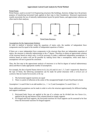
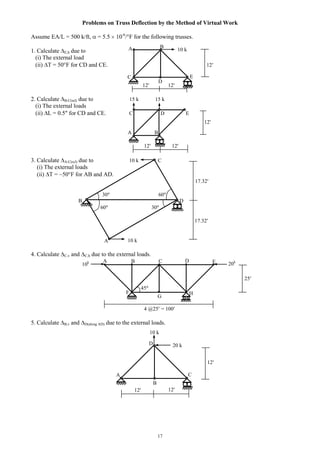
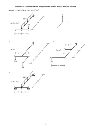
![4
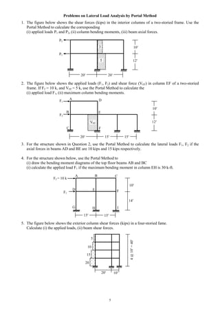
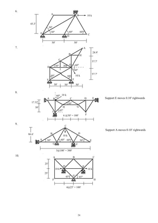
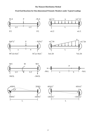
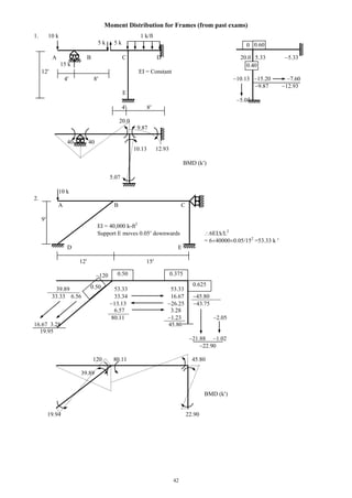
Analysis of Multi-storied Structures by Portal Method
Approximate methods of analyzing multi-storied structures are important because such structures are
statically highly indeterminate. The number of assumptions that must be made to permit an analysis by
statics alone is equal to the degree of statical indeterminacy of the structure.
Assumptions
The assumptions used in the approximate analysis of portal frames can be extended for the lateral load
analysis of multi-storied structures. The Portal Method thus formulated is based on three assumptions
1. The shear force in an interior column is twice the shear force in an exterior column.
2. There is a point of inflection at the center of each column.
3. There is a point of inflection at the center of each beam.
Assumption 1 is based on assuming the interior columns to be formed by columns of two adjacent bays or
portals. Assumption 2 and 3 are based on observing the deflected shape of the structure.
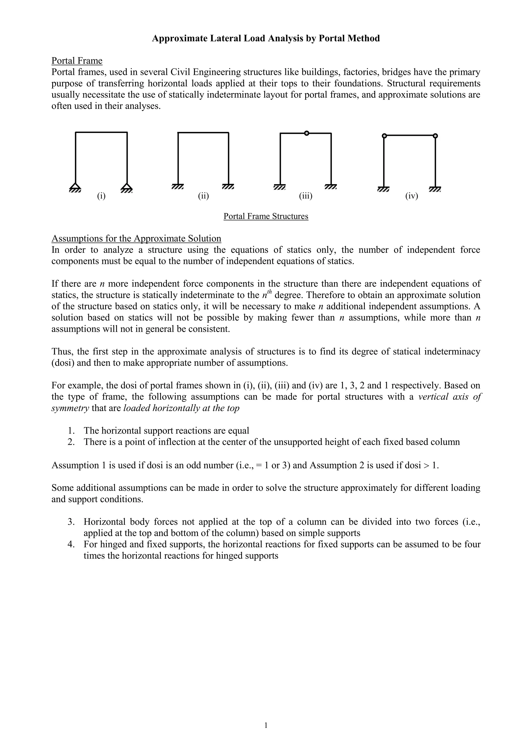
Example
Use the Portal Method to draw the axial force, shear force and bending moment diagrams of the three-storied
frame structure loaded as shown below.
E
A
404040
151515
33
15 10 15
18k
12k
6k
122@10=20
Beam BMD (k-ft) Beam SFD (k) Column AFD (k)
616161
-3-2 -2
-8
-5.33 -5.33
-2
-3.67
12
-7.75
3.67
-1
7.7515.5
-7.33
-12.2-8.13 -8.13
12
10
6
12
10
6
6 6
55
Column shear forces are at the ratio of 1:2:2:1.
Shear force in (V) columns IM, JN, KO, LP are
[18 1/(1 + 2 + 2 + 1) =] 3k
, [18 2/(1 + 2 + 2 + 1) =] 6k
,
6k
, 3k
respectively. Similarly,
VEI = 30 1/(6) = 5k
, VFJ = 10k
, VGK = 10k
, VHL = 5k
; and
VAE = 36 1/(6) = 6k
, VBF = 12k
, VCG = 12k
, VDH = 6k
Bending moments are
MIM = 3 10/2 = 15k
, MJN = 30k
, MKO = 30k
, MLP = 15k
MEI = 5 10/2 = 25k
, MFJ = 50k
, MGK = 50k
, MHL = 25k
MAE = 6 10/2 = 30k
, MFJ = 60k
, MGK = 60k
, MHL = 30k
M
I
F
B
N
J
G
C
O
K
H
P
L
D
The rest of the calculations follow from the free-body diagrams
72
50
30
25
15
36
25
15
3672
50
30
Column SFD (k) Column BMD (k-ft) Beam AFD (k)
-15 -9 -3
-10
-6 -2
-5 -3 -1
-15.5
7.33](https://image.slidesharecdn.com/structuralengineeringii1-160123221338/85/Structural-engineering-ii-4-320.jpg)
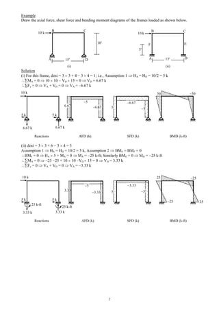
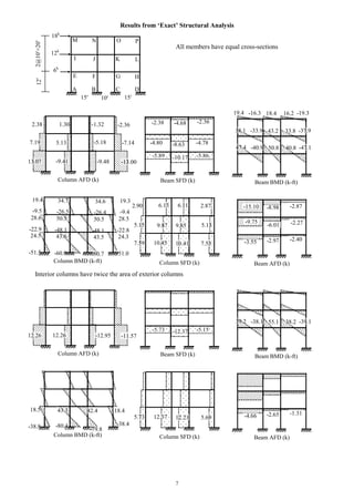
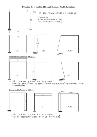
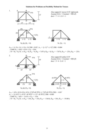
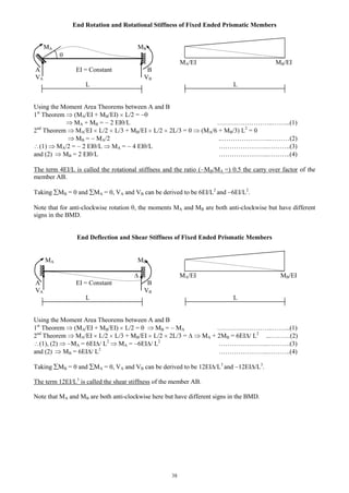
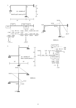
![6
Analysis of Multi-storied Structures by Cantilever Method
Although the results using the Portal Method are reasonable in most cases, the method suffers due to the
lack of consideration given to the variation of structural response due to the difference between sectional
properties of various members. The Cantilever Method attempts to rectify this limitation by considering the
cross-sectional areas of columns in distributing the axial forces in various columns of a story.
Assumptions
The Cantilever Method is based on three assumptions
1. The axial force in each column of a storey is proportional to its horizontal distance from the
centroidal axis of all the columns of the storey.
2. There is a point of inflection at the center of each column.
3. There is a point of inflection at the center of each beam.
Assumption 1 is based on assuming that the axial stresses can be obtained by a method analogous to that
used for determining the distribution of normal stresses on a transverse section of a cantilever beam.
Assumption 2 and 3 are based on observing the deflected shape of the structure.
Example
Use the Cantilever Method to draw the axial force, shear force and bending moment diagrams of the three -
storied frame structure loaded as shown below.
E
A
15 5 5 15
18k
12k
6k
122@10=20
42.435.342.4
15.913.215.9
Beam BMD (k-ft)
64.653.864.6
The dotted line is the column centerline (at all floors)
Column axial forces are at the ratio of 20: 5: 5: 20.
Axial force in (P) columns IM, JN, KO, LP are
[18 5 20/{202
+ 52
+ ( 5)2
+ ( 20)2
} = ] 2.12k
, [18 5
5/(202
+ 52
+ ( 5)2
+ ( 20)2
} = ] 0.53k
, 0.53k
, 2.12k
respectively.
Similarly, PEI = 330 20/(850) = 7.76k
, PFJ = 1.94k
, PGK =
1.94k
, PHL = 7.76k
; and
PAE = 696 20/(850) = 16.38k
, PBF = 4.09k
, PCG = 4.09k
,
PDH = 16.38k
M
I
F
B
N
J
G
C
O
K
H
P
L
D
The rest of the calculations follow from the free-body diagrams
Beam AFD (k)
-14.82 -8.98 -3.04
-9.88
-6.00 -2.12
-4.95 -3.00 -1.05
Beam SFD (k)
-2.65-2.12 -2.12
-7.06-5.65 -5.64
-10.76-8.61 -8.61
-7.76
-2.12
-1.94
-0.532.12
1.94
0.53
7.76
Column AFD (k)
16.38 -16.38
Column BMD (k-ft)
69.9
1
48.5
29.1
26.5
15.9
38.1
26.5
15.9
38.169.9
48.5
29.1
4.09 -4.09
3.18
Column SFD (k)
5.825.82 3.18
11.65
9.70
11.65
9.70
6.35 6.35
5.305.30](https://image.slidesharecdn.com/structuralengineeringii1-160123221338/85/Structural-engineering-ii-6-320.jpg)
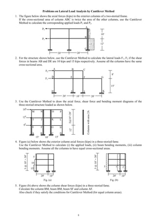
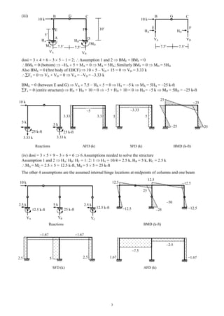
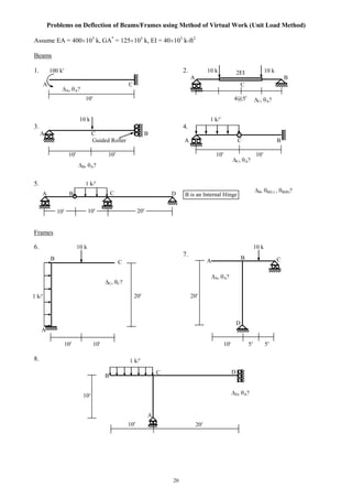
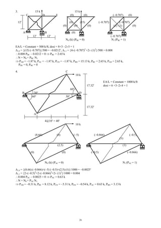
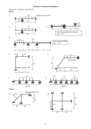
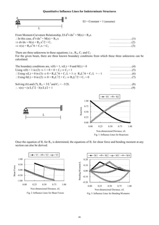
![9
Approximate Vertical Load Analysis
Approximation based on the Location of Hinges
If a beam AB is subjected to a uniformly distributed vertical load of w per unit length [Fig. (a)], both the
joints A and B will rotate as shown in Fig. (b), because although the joints A and B are partly restrained
against rotation, the restraint is not complete. Had the joints A and B been completely fixed against rotation
[Fig. (c)] the points of inflection would be located at a distance 0.21L from each end. If, on the other hand,
the joints A and B are hinged [Fig. (d)], the points of zero moment would be at the end of the beam. For the
actual case of partial fixity, the points of inflection can be assumed to be somewhere between 0.21 L and 0
from the end of the beam. For approximate analysis, they are often assumed to be located at one-tenth (0.1
L) of the span length from each end joint.
(a) (b) (c) (d)
Depending on the support conditions (i.e., hinge ended, fixed ended or continuous), a beam in general can be
statically indeterminate up to a degree of three. Therefore, to make it statically determinate, the following
three assumptions are often made in the vertical load analysis of a beam
1. The axial force in the beam is zero
2. Points of inflection occur at the distance 0.1 L measured along the span from the left and right support.
Bending Moment and Shear Force from Approximate Analysis
Based on the approximations mentioned (i.e., points of inflection at a distance 0.1 L from the ends), the
maximum positive bending moment in the beam is calculated to be
M(+) = w(0.8L)2
/8 = 0.08 wL2
, at the midspan of the beam
The maximum negative bending moment is
M( ) = wL2
/8 0.08 wL2
= 0.045 wL2
, at the joints A and B of the beam
The shear forces are maximum (positive or negative) at the joints A and B and are calculated to be
VA = wL/2, and VB = wL/2
Moment and Shear Values using ACI Coefficients
Maximum allowable LL/DL = 3, maximum allowable adjacent span difference = 20%
1. Positive Moments
(i) For End Spans
(a) If discontinuous end is unrestrained, M(+) = wL2
/11
(b) If discontinuous end is restrained, M(+) = wL2
/14
(ii) For Interior Spans, M(+) = wL2
/16
2. Negative Moments
(i) At the exterior face of first interior supports
(a) Two spans, M( ) = wL2
/9
(b) More than two spans, M( ) = wL2
/10
(ii) At the other faces of interior supports, M( ) = wL2
/11
(iii) For spans not exceeding 10 , of where columns are much stiffer than beams, M( ) = wL2
/12
(iv) At the interior faces of exterior supports
(a) If the support is a beam, M( ) = wL2
/24
(b) If the support is a column, M( ) = wL2
/16
3. Shear Forces
(i) In end members at first interior support, V = 1.15wL/2
(ii) At all other supports, V = wL/2
[where L = clear span for M(+) and V, and average of two adjacent clear spans for M( )]
0.21L0.21L
DCDC
BABABA
BA
L
k2Lk1L](https://image.slidesharecdn.com/structuralengineeringii1-160123221338/85/Structural-engineering-ii-9-320.jpg)
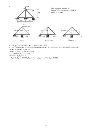
![15
Deflection Calculation by the Method of Virtual Work
Method of Virtual Work
Another way of representing the equilibrium equations is by energy methods, which is based on the law of
conservation of energy. According to the principle of virtual work, if a system in equilibrium is subjected to
virtual displacements, the virtual work done by the external forces ( WE) is equal to the virtual work done
by the internal forces ( WI)
WE = WI …...…………………(1)
where the symbol is used to indicate ‘virtual’. This term is used to indicate hypothetical increments of
displacements and works that are assumed to happen in order to formulate the problem.
while the virtual work done by the virtual internal force (u) on B is = u. dL …...…………………(3)
The total internal virtual work done is WI = u. dL …...…………………(4)
where the symbol indicates the summation over the lengths of all the elements within the body.
In this formulation, the terms in italic indicate virtual loads or internal forces.
The principle of virtual work [Eq. (1)] 1. = u. dL = u. dL …...…………………(5)
It is to be noted here that the term above can indicate the deflection or rotation of the body, depending on
which the virtual load (1) can be a unit force or a unit moment applied in the direction of .
Deflection of Truss due to External Loads
The above principle can be applied to calculate the deflection of a truss due to axial deformation of its
members. This axial deformation can be caused be caused by external loads on the truss, temperature change
or misfit of member length. The axial deformation due to external loads is caused by the internal forces
within the truss members, the resulting extension of a truss member being
dL = N0L/EA …...…………………(6)
where N0, L, E and A stand for the axial force (due to external loads), length, modulus of elasticity and
cross-sectional area of a truss member. The internal force u due to the unit virtual load is often expressed by
N1, from which the equation for truss deflection [Eq. (5)] becomes = N1. N0L/EA ……….……(7)
Example
Calculate the vertical deflection of the point B of the truss ABCDEF due to the external loads applied
[Given: EA/L = 500 kip/ft, for all the truss members].
Using member forces N0 and N1 from the above analyses, = N0 N1 L/EA ……….……(7)
Ignoring zero force members,
B,v = {(7.07) (0.707) + (−7.07) (0.707) + (−5) (−0.5) + (−5) (−0.5)}/500 = 0.01 ft
Consider the body loaded as shown in Fig. 1. Under the given
loading conditions, the point A deflects an amount in the direction
shown in the Figure. Moreover the same load causes the element B
within the body to extend an amount dL in the direction shown.
If a virtual unit load (i.e., a load of magnitude 1), when applied in
the direction of , causes a virtual internal force u in the element B
in the direction of dL, the virtual work done by the external forces
WE = 1. …...…………………(2)
Fig. 1
A
B
dL
u
1
A B C
F E D
A B C
F E D
A B
C
F E D
3 @ 20 = 60
20
10 k
0
0
1010
-14.147.07 -7.07
-5 -5
N0 (k) N1
10 k
1
-10.707 0.707
-0.5 -0.5
0 0
0
0](https://image.slidesharecdn.com/structuralengineeringii1-160123221338/85/Structural-engineering-ii-15-320.jpg)
![16
Deflection of Truss due to Temperature Change and Misfit
In addition to external loads, a truss joint may deflect due to change in member lengths (i.e., become longer
or shorter than its original length) caused by change in temperature or geometrical misfit of any truss
member (being longer or shorter than its specified length).
In Eq. (5); i.e., = u. dL …...…………………(5)
the tem dL (elongation of a truss member) can also be due to temperature change or fabrication defect of any
truss member.
The change in length due to increase in the temperature T is = T L …...…………………(8)
where = Coefficient of thermal expansion; i.e., change of length of a member of unit length due to unit
change of temperature, T = Change of temperature of a member of length L.
Adding to it a geometric misfit (due to fabrication defect) of L, the total elongation of a truss member
dL = N0L/EA + T L + L …...…………………(9)
from which the equation for truss deflection [Eq. (5)] becomes
= N1 dL = N1 (N0L/EA + T L + L) …...…………………(10)
Example
Calculate the vertical deflection of joint B of the truss ABCDEF shown below due to
(i) temperature rise of 30 F in the bottom cord members AB and BC,
(ii) fabrication defects resulting in vertical members BF and CE to be made 0.25 shorter than specified
[Given: Coefficient of thermal expansion = 5.5 10-6
/ F, for all the truss members].
(i) For members AB and BC, = 5.5 10-6
/ F, T = 30 F, L = 20 ft = 240 in
dL = T L = (5.5 10-6
) (30) (240) = 0.0396 in
Ignoring zero force members, B,v = (0.0396) (-0.5) + (0.0396) (-0.5) = 0.0396 in
(ii) For members BF and CE, dL = 0.25 in
Ignoring zero force members, B,v = ( 0.25) (-1) + ( 0.25) (0) = 0.25 in
Support Settlement
Settlement of supports due to consolidation or instability of the subsoil/foundation is a major reason of
deflection of structures. There is a fundamental difference between the effect of support settlement on
statically determinate and indeterminate structures. While it causes deflection due to geometrical changes
only in statically determinate structures, it induces internal stresses in statically indeterminate structures
(which may even be more significant than the forces due to external loads).
The effect of support settlement on statically indeterminate structures is dealt separately but the following
figure shows the deflected shape of the truss ABCDEF shown above due to settlement of support C.
A
B
C
F E D
3 @ 20 = 60
20 -0.25
-0.25
0.0396
dL (in) N1
1
-10.707 0.707
-0.5 -0.5
0 0
0
0
0.0396](https://image.slidesharecdn.com/structuralengineeringii1-160123221338/85/Structural-engineering-ii-16-320.jpg)
![18
Deflection due to Flexural Deformations
Flexural deformation is the main source of deflection in many civil engineering structures, like beams, slabs
and frames; i.e., those designed primarily against bending moment. It is often much more significant than
other causes of deflection like axial, shear and torsional deformation. From Eq. (5) of the previous section,
the principle of virtual work = u. dL …………………(5)
where the term above can indicate the deflection or rotation of the body, u is the virtual internal force in
an element within the body, which deforms by an amount dL in the direction of u.
Deflection of Beam/Frame due to External Loads
For flexural deformation, u is be the virtual internal moment m1 in the element while dL is the rotation d
caused by external forces; i.e., dL = d = curvature ds = (m0/EI) ds.
= m1 m0/EI ds …………………(11)
where m0 is the bending moment caused by external forces and EI is called the flexural rigidity of the
member. Here, the integration sign is used instead of summation because the bending moments vary
within the length of each member (unlike the trusses, where axial forces do not vary within the members).
Integration Table
In order to facilitate the integration shown in Eq. (11), the following table is used between functions f1 and
f2, both of which can be uniform or vary linearly or parabolically along the length (L) of a member.
Integration of Product of Functions (I = f1 f2 dS)
f2 f1 A
L
B
L
A
L
A B
L
A C B
L
a
L
AaL BaL/2 AaL/2 (A+B)aL/2 [A+4C+B]aL/6
b
L
AbL/2 BbL/3 AbL/6 [A+2B]bL/6 [2C+B]bL/6
a
L
AaL/2 BaL/6 AaL/3 [2A+B]aL/6 [A+2C]aL/6
a b
L
A(a+b)L/2 B(a+2b)L/6 A(2a+b)L/6 [A(2a+b)+B(a+2b)]L/6
[Aa+Bb+
2C(a+b)]L/6
Example: Calculate the tip rotation and deflection of the beam shown below [Given: EI = const].
m1
m0
B
P0L
A
P0
L
L
1
m1
Using the m0 diagram along with m1 for unit anticlockwise
moment at A
A = ( 1) ( P0L/EI) L/2 = P0L2
/2EI
Using the m0 diagram and m1 for unit upward load at A
vA = (L) ( P0L/EI) L/3 = P0L3
/3EI](https://image.slidesharecdn.com/structuralengineeringii1-160123221338/85/Structural-engineering-ii-18-320.jpg)

![22
Flexibility Method for 2-degree Indeterminate Trusses
D C 10 k
EA/L = constant = 1000 k/ft
(Note: EA constant)
dosi = 1 6 + 4 – 2 4 = 2
10 The horizontal reaction HB and member force FBD
are taken as the two redundants.
A B
10
10 k
1,0 = {N1 N0 /(EA/L)} = {0 0 + 0 0 + 0 14.14 + 0 (–10) + 1 0}/1000 = 0 ft
2,0 = {N2 N0 /(EA/L)} = {14.14 1 + (–10) (–0.707)}/1000 = 21.21 10-3
ft
1,1 = {N1 N1 /(EA/L)} = {02
+ 02
+ 02
+ 02
+ 12
}/1000 = 1 10-3
ft/k
1,2 = 2,1 = {N1 N2 /(EA/L)} = {1 (–0.707)}/1000 = –0.707 10-3
ft/k
2,2 = {N2 N2 /(EA/L)} = {4 (–0.707)2
+ 2 12
}/1000 = 4 10-3
ft/k
(1 10-3
) HB + (–0.707 10-3
) FBD = 0
(–0.707 10-3
) HB + (4 10-3
) FBD = –21.21 10-3
HB = – 4.29 k, and FBD = – 6.06 k
N = N0 + N1 HB + N2 FBD
FAB = 0 +1 (– 4.29) + (–0.707) (–6.06) = 0, FBC = –10 + 0 + (–0.707) (–6.06) = –5.71 k
FCD = 0 +0 + (–0.707) (–6.06) = 4.29, FDA = 0 +0 + (–0.707) (–6.06) = 4.29 k
FAC = 14.14 + 0 +(1) (–6.06) = 8.08 k, FBD = – 6.06 k
(0)
(0)
(0)
(14.14) ( 10) (0)
(0)
(0) (0)
(1)
(1)
( 0.707)
(1)
( 0.707)
( 0.707)
( 0.707)
Case 0 (HB = 0, FBD = 0)
[Forces N0 (k)]
Case 1 (HB = 1)
[Forces N1]
Case 2 (FBD = 1)
[Forces N2]](https://image.slidesharecdn.com/structuralengineeringii1-160123221338/85/Structural-engineering-ii-22-320.jpg)
![28
Flexibility Method for 1-degree Indeterminate Beams
Example 1
EI = constant
A B C dosi = 3 1 + 4 – 3 2 = 1
Take RA as the redundant
L/2 L/2 1,0 + RA 1,1 = A = 0 …………..…(i)
1,0 = (L/2)/6 [2L + L/2] (–PL/2)/EI = – 5PL3
/48EI
1,1 = m1 m1 dS/EI
= L/3 (L) (L)/EI = L3
/3EI
m1
(i) – 5PL 3
/48EI + L3
/3EI = 0 RA = 5P/16
M = m0 + RA m1 = m0 + (5P/16) m1
M MA = 0, MB = 5PL/32, MC = –PL/2 + 5PL/16 = –3PL/16
Example 2
EI = constant
A B C dosi = 3 2 + 4 – 3 3 = 1
Take RB as the redundant
10 10 1,0 + RB 1,1 = B = 0 …………..…(i)
1,0 = 2 [2 37.5 + 50] (–5 10/6)/EI = –2083.33/EI
1,1 = m1 m1 dS/EI
m1 ( ) = 2 10/3 (–5) (–5)/EI = 166.67/EI
– 5 (i) –2083.33/EI + 166.67 RB/EI = 0
RB = 12.5 k
M = m0 + RB m1 = m0 + 12.5 m1
M (k ) MA = 0, MB = 50 – 62.5 = – 12.5 k , MC = 0
– 12.5
6.256.25
1 k/ft
m0 (k )
37.5
50
P
m0
PL/2
100
L
L/2
3PL/16
5PL/32](https://image.slidesharecdn.com/structuralengineeringii1-160123221338/85/Structural-engineering-ii-28-320.jpg)
![29
Flexibility Method for 2-degree Indeterminate Beams
Example 3
10 k 10 k
A B C D E
dosi = 3 2 + 5 – 3 3 = 2
EI = 1 EI = 1 1,0 + RA 1,1 + RC 1,2 = A = 0 ……(i)
5 5 5 5 2,0 + RA 2,1 + RC 2,2 = C = 0 ……(ii)
m0 (k ) 1,0 = m1 m0 dS/EI
0 0 = {10/6 (–100) (30+5)
–50 –100 + 5/6[(–100)(30+20) + (–200)(40+15)]}/EI
–200 = –19166.67/EI
15 20 2,0 = m2 m0 dS/EI
5 = {5/6 (5) (–200–50)
m1 ( ) + 5/6 [(5)(–200–200)+(10)(–400–100)]}/EI = – 6875/EI
1,1 = m1 m1 dS/EI = 20/3 (20) (20)/EI
= 2666.67/EI
5 10 1,2 = 2,1 = m1 m2 dS/EI
m2 ( ) = {5/6(5)(30+10)
+5/6 [(5)(30+20)+(10)(40+15)]}/EI
= 833.33/EI
2,2 = m2 m2dS/EI = 10/3 (10) (10)/EI
= 333.33/EI
Avoiding the factors EI
(i) 2666.67 RA + 833.33 RC = 19166.67
(ii) 833.33 RA + 333.33 RC = 6875
RA = [19166.67 333.33 – 833.33 6875]/[2666.67 333.33 – 833.332
] = 3.39 k
and RC = [2666.67 6875 – 833.33 19166.67]/[2666.67 333.33 – 833.332
] = 12.14 k
M = m0 + RA m1 + RC m2 = m0 + 3.39 m1 + 12.14 m2
MA = 0, MB = 0 + 3.39 5+ 0 12.14 = 16.95 k , MC = –50 + 3.39 10 +0 12.14 = –16.10 k ,
MD = –100 + 3.39 15 + 5 12.14 = 11.55 k , ME = –200 + 3.39 20 + 10 12.14 = –10.80 k
16.95
11.55
M (k )
10
–16.10
–10.80](https://image.slidesharecdn.com/structuralengineeringii1-160123221338/85/Structural-engineering-ii-29-320.jpg)
![30
Analysis for Support Settlement
Example 4
Support B settles 0.10
A B C EI = 40 103
k-ft2
dosi = 3 2 + 4 – 3 3 = 1
1,0 + RB 1,1 = B = –0.10 ……(i)
10 10 1,0 = 0
m1 ( ) 1,1 = m1 m1 dS/EI
= 2 10/3 (–5) (–5)/EI = 166.67/40 103
–5 (i) 166.67 RB/40 103
+ 0 = –0.10
RB = – 4000/166.67 = –24 k
120
M = m0 + RB m1 = –24 m1 [in k ]
M (k )
Example 5
Support C settles 0.10
EI = 40 103
k-ft2
A B C D E dosi = 2
1,0 + RA 1,1 + RC 1,2 = A = 0.…..….(i)
10 10 2,0 + RA 2,1 + RC 2,2 = C = –0.10.…(ii)
1,0 = 0, 2,0 = 0
1,1 = m1 m1 dS/EI = 2666.67/EI, 1,2 = 2,1 = 833.33/EI, 2,2 = 333.33/EI
(i) (2666.67/EI) RA + (833.33/EI) RC = 0
(ii) (833.33/EI) RA + (333.33/EI) RC = –0.10
RA = 17.14 k, and RC = –54.86 k
M = m0 + RA m1 + RC m2 = 17.14 m1 – 54.86 m2 [in k ]
MA = 0, MB = 17.14 5 – 0 54.86 = 85.70, MC = 17.14 10 – 0 54.86 = 171.40,
MD = 17.14 15 – 5 54.86 = –17.20, ME = 17.14 20 – 10 54.86 = – 205.80
171.40
M (k )
–205.80](https://image.slidesharecdn.com/structuralengineeringii1-160123221338/85/Structural-engineering-ii-30-320.jpg)
![31
Combined Flexural, Shear and Axial Deformations
B C
EA = 400 103
k, GA*
= 125 103
k
EI = 40 103
k-ft2
dosi = 3 3 + 4 – 3 4 = 1
10
The vertical reaction at D (VD) is taken
as the redundant.
A D
10
–10
–10
100
x0 (k) v0 (k) m0 (k )
10
–1
–1
x1 v1 m1 ( )
1,0 = (x1 x0/EA) dS + (v1 v0 /GA*
) dS + (m1 m0 /EI) dS
= 0 + 0 + 10/2 (100)(10)/(40 103
) = 0.125 ft
1,1 = (x1 x1/EA) dS + (v1 v1 /GA*
) dS + (m1 m1 /EI) dS
= 2 10 (1 1)/(400 103
)+10 (1 1)/(125 103
)+[10 (10 10)+10 (10 10)/3]/(40 103
)
= 0.05 10–3
+ 0.08 10–3
+33.33 10–3
= 33.46 10–3
VD = –0.125/33.46 10–3
= –3.74 k
1
10 k](https://image.slidesharecdn.com/structuralengineeringii1-160123221338/85/Structural-engineering-ii-31-320.jpg)
![34
5. dosi = 9 + 5 – 12 – 1 = 1; i.e., assume RC as the redundant
1,0 = (m0 m1/EI) dS = 10/6 (–50–2 100) (10)/(40 103
) = –0.1042 ft
1,1 = (m1 m1/EI) dS = 10/3 (10) (10)/(40 103
) = 8.33 10–3
ft/k
RB = 0.1042/(8.33 10–3
) = 12.5 k
6. dosi = 6 + 5 – 9 = 2; i.e., assume RB and MC as the redundants
1,0 = –0.0521 ft, 1,1 = 4.17 10–3
ft/k (as in Problem 4)
2,0 = (m0 m2/EI) dS = 20/6 (2 50+0) (1)/(40 103
) = 8.33 10–3
rad
1,2 = 2,1 = (m1 m2/EI) dS = {10/3 (–5)(0.5) +10/6 (–5)(1+2 0.5)}/(40 103
) = –0.625 10-3
rad/k
2,2 = (m2 m2/EI) dS = 20/3 (1)(1)/(40 103
) = 0.167 10-3
rad/k-ft
4.17 RB – 0.625 MC = 52.1; and –0.625 RB + 0.167 MC = –8.33
RB = 11.43 k, MC = –7.14 k-ft
7. dosi = 6 + 5 – 9 = 2; i.e., assume RB and RC as the redundants
1,0 = (m0 m1/EI) dS
= {5/3(50)(3.33)+5/2(50)(3.33+6.67)+15/2(50)(6.67+1.67)+5/3(50)(1.67)}/(40 103
)= 119.8 10–3
ft
1,1 = (m1 m1/EI) dS = {10/3 ( 6.67) ( 6.67) + 20/3 ( 6.67) ( 6.67)}/(40 103
) = 11.11 10–3
ft/k
1,2 = 2,1 = (m1 m2/EI) dS = [10/3( 6.67)( 3.33) + 10/6{( 6.67)( 2 3.33 6.67)
+( 3.33)( 2 6.67 3.33)}+10/3( 6.67)( 3.33)]/(40 103
) = 9.72 10–3
ft/k
2,0 = 1,0 = 119.8 10–3
ft, 2,2 = 1,1 = 11.11 10–3
ft/k
RB = RC = 5.75 k (i.e., upward)
–7.14
7.5
21.25
0.5 1
100
10
m0 (k )
37.5
50
m1 ( )
RB = 1
–5
1.347.14
–10.71
M (k )
RC = 1
m1 ( )
25
–50
M (k )
25
m0 (k )
50
25
m2
MC = 1
M (k )
6.67m0 (k )
50
6.67
50
RB = 1
m1 ( )
RC = 1
m2 ( )](https://image.slidesharecdn.com/structuralengineeringii1-160123221338/85/Structural-engineering-ii-34-320.jpg)
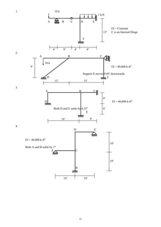
![39
Rotation of a Joint and Moment Distribution Factors (MDF)
B
A KOB
KOA MO
O KOC C
KOE
E
KOD
D
Flexural members OA, OB, OC…...are joined at joint O and have rotational stiffnesses of KOA, KOB,
KOC…….respectively; i.e., for unit rotation of the joint O they require moments KOA, KOB, KOC…….
respectively to be applied at O.
If a moment MO applied at joint O causes it to rotate by an angle , the following moments are needed to
rotate members OA, OB, OC…...
MOA = KOA ………..(1)
MOB = KOB ………..(2)
MOC = KOC ………..(3)
………………………
Adding (1), (2), (3)…. MOA + MOB + MOC + …….= KOA + KOB + KOC +…… ………..(4)
Since MO = MOA + MOB + MOC + ……….
MO = (KOA + KOB + KOC +……) = KO [KO = KOA + KOB + KOC +……]
= MO/(KO) ………..(5)
(1) MOA = [KOA/KO] MO ………..(6)
(2) MOB = [KOB/KO] MO ………..(7)
(3) MOC = [KOC/KO] MO ………..(8)
………………………
The factors [KOA/KO], [KOB/KO], [KOC/KO]………..are the moment distribution factors (MDF) of members
OA, OB, OC……..respectively. Therefore the distributed moments in members are proportional to their
respective MDFs.
Example
10 k
0.60 12.5 12.5 3.75 7.5 16.25
0.40 5.0 5.0
15
EI = Constant
2.5
5 5
[Load and MDF] [FEM] [Dist M] [Total end M]
5.0
2.5](https://image.slidesharecdn.com/structuralengineeringii1-160123221338/85/Structural-engineering-ii-39-320.jpg)
![44
Qualitative Influence Lines and Maximum Forces
1. For the beam shown below, draw the influence lines of RA, RB, VB
(L)
, VB
(R)
, MA, MB.
A B C
10 5
RA RB
VB
(L)
VB
(R)
MA MB
2. For the beam shown below, DL = 1 k/ , moving LL = 0.5 k/ (UDL), 5 k (concentrated).
Calculate the maximum values of RA, RB, ME, MB and MF [Each span is 10 long].
A B C D A B C D
E F G (RA) E F G (RB)
A B C D A B C D
E F G (ME) E F G (MB)
1.5 k/ 5 k
1 k/ 1 k/
(MF) Load arrangement for MF(max)
Final end moments 0 16.25 16.25
MF(max) = 16.25 + 1.5 102
/8 + 5 10/4 = 15 k](https://image.slidesharecdn.com/structuralengineeringii1-160123221338/85/Structural-engineering-ii-44-320.jpg)
![45
3. For the beam shown below, draw the qualitative influence lines for
(i) Bending moments MC, MD, ME, MF
(ii) Support reactions RB, RD, RE, RF
(iii) Shear forces VB
(R)
, VD
(L)
, VD
(R)
, VE
(L)
, VE
(R)
,VF
If the beam is subjected to a uniformly distributed DL = 1.5 k/ft and moving LL = 0.5 k/ft (uniformly
distributed) and 5 k (concentrated), calculate the maximum values of
(i) positive MC, (ii) positive RD and (iii) positive VE
(R)
[Given: EI = constant].
A B C D E F
5 5 5 10 10
IL of MC IL of RD IL of VE
(R)
IL of MD IL of RF IL of VD
(L)
(i) Maximum positive value of MC: (ii) Maximum positive value of RD:
5 k 5 k
1.5 k/ 2 k/ 1.5 k/ 2 k/ UDL 1.5 k/ 2 k/ 2 k/ 1.5 k/
0 1 3/7 4/7 0.5 0.5 DF 0 1 3/7 4/7 0.5 0.5
18.75 22.92 22.92 12.5 12.5 16.67 16.67 FEM
( 4.17) (2.08) (2.08) (2.08)
2.08
(5.36) (7.14) 3.57 ( 0.89) ( 1.19) 0.60
1.93 ( 3.87) ( 3.87) 1.93
(0.83) (1.10) 0.55 ( 0.06) ( 0.09)
0.14 ( 0.27) ( 0.28) 0.14
(0.06) (0.08)
18.75 18.75 18.75 18.75 12.52 12.52 18.74 VD
(L)
= 2 10/2+(18.75 16.58)/10= 9.78 k
VD
(R)
= 2 10/2+(16.58 14.88)/10 = 10.17 k
Maximum value of MC Maximum RD = VD
(R)
VD
(L)
+5 =24.95 k
= 18.75 + 2 102
/8 + 5 10/4 = 18.75 k
18.75 16.67 16.67 16.67 16.66 12.5 12.5
1.04 1.04 1.04
0.15 (0.30) (0.30) 0.15
18.75 18.75 16.58 16.58 14.88 14.88 11.31](https://image.slidesharecdn.com/structuralengineeringii1-160123221338/85/Structural-engineering-ii-45-320.jpg)
![48
Non-coplanar Forces and Analysis of Space Truss
Non-coplanar Force
A vector in space may be defined or located by any three mutually perpendicular reference axes Ox, Oy and
Oz (Fig. 1). This vector may be resolved into three components parallel to the three reference axes.
Space Truss
Although simplified two-dimensional structural models are quite common, all civil engineering structures
are actually three-dimensional. Among them, electric towers, offshore rigs, rooftops of large open spaces
like industries or auditoriums are common examples of three-dimensional or space truss. The members of a
space truss are non-coplanar and therefore their axial forces can be modeled as non-coplanar forces.
Since there is only one force per member and three equilibrium equations per joint of a space truss, the
degree of statical indeterminacy (dosi) of such a structure is given by
dosi = m + r 3j ……………………………(viii)
The three equilibrium equations per joint of a space truss are related to forces in the three perpendicular axes
x, y and z
Fx = 0, Fy = 0 and Fz = 0 ……..………………………(ix)
However the other three equilibrium equations related to moments; i.e.,
Mx = 0, My = 0 and Mz = 0 ……..………………….……(x)
may also be needed to calculate the support reactions of the truss. Here, it is pertinent to mention that the
moment of a force about an axis is zero if the force is parallel to the axis (when it does not produce any
rotational tendency about that axis) or intersects it (when the perpendicular distance from the axis is zero).
If the force OC (of magnitude F) makes angles , and
with the three reference axes Ox, Oy and Oz, then the
components of the force along these axes are given by
Fx = F cos …….……….……….………(i)
Fy = F cos …...……….…………..…….(ii)
Fz = F cos …….……..…………..……(iii)
[(i)2
+ (ii)2
+ (iii)2
] F = [Fx
2
+ Fy
2
+ Fz
2
] ….…...….(iv)
(i) cos = Fx/ [Fx
2
+ Fy
2
+ Fz
2
] …….…….……(v)
(ii) cos = Fy/ [Fx
2
+ Fy
2
+ Fz
2
] ……….…..…...(vi)
(iii) cos = Fz/ [Fx
2
+ Fy
2
+ Fz
2
] ……….…..….(vii)
The values of cos , cos and cos given by Eqs. (v), (vi)
and (vii) are called the direction cosines of the vector F.
C
z
xO
y
Fig. 1: Non-coplanar Force and Components](https://image.slidesharecdn.com/structuralengineeringii1-160123221338/85/Structural-engineering-ii-48-320.jpg)
![49
Example: Calculate the support reactions and member forces of the truss shown below.
MCD = 0 YA 20 10 20 = 0 YA = 10 k ….…………(1)
MBC = 0 YA 30 + YD 30 + 20 25 = 0 YD = 26.67 k …………….(2)
My(D) = 0 20 10 + ZC 30 = 0 ZC = 6.67 k ………….…(3)
Fy = 0 YA + YC + YD 10 = 0 YC = 26.67 k …...………..(4)
Fx = 0 XD + XC + 20 = 0 …………….(5)
Fz = 0 ZD + ZC = 0
ZD = ZC = 6.67 k [using (3)] ……………..(6)
Equilibrium of Joint A (unknowns FAB, FAD and FAE):
Fx = 0 FAB + 0.49 FAE = 0 …………..…(7)
Fy = 0 0.81 FAE + 10 = 0 FAE = 12.33 k …..………....(8)
FAB = 0.49 FAE = 6.00 k [using (7)] …..………....(9)
Fz = 0 FAD 0.32 FAE = 0 FAD = 4.00 k [using (8)] …....………(10)
Equilibrium of Joint B (unknowns FBC, FBD and FBE):
Fx = 0 FBA 0.83 FBD 0.49 FBE = 0 ……………(11)
Fy = 0 0.81 FBE 10 = 0 FBE = 12.33 k …...……….(12)
FBD = ( FBA 0.49 FBE)/0.83 = 14.42 k [using (11)] …...……….(13)
Fz = 0 FBC 0.56 FBD 0.32 FBE = 0 FBC = 4.00 k [using (12), (13)] ….…..….…(14)
Equilibrium of Joint C (unknowns XC and FCE):
Fx = 0 XC 0.49 FCE = 0 …………….(15)
Fy = 0 26.67 + 0.81 FCE = 0 FCE = 32.88 k ………….…(16)
XC = 0.49 FCE = 16 k [using (16)] …...……..…(17)
Fz = 0 6.67 + 0.32 FCE + FCB = 0 FCB = 4.00 k [verified]
Equilibrium of Joint D (unknowns XD and FDE):
Fx = 0 XD + 0.49 FDE + 0.83 FDB = 0 ……………...(18)
Fy = 0 26.67 + 0.81 FDE = 0 FDE = 32.88 k …..………….(19)
XD = 4.00 [using (13), (19)] ……...………(20)
XC = 20 XD = 16.00 [using (5)] …...…………(21)
Fz = 0 6.67 + 0.32 FDE + FDA + 0.56 FDB = 0 6.67 + 10.67 + 4.00 8.00 = 0
0 = 0 [verified]
z
y
10 k
20 kE
CD
B
A
25
10
Ignoring the zero force member CD
dosi = m + r 3j = 8 + 7 3 5 = 0
The structure is statically determinate.
Member Lx Ly Lz Cx Cy Cz
AB 30 0 0 1.00 0.00 0.00
BC 0 0 20 0.00 0.00 1.00
BD 30 0 20 0.83 0.00 0.56
AD 0 0 20 0.00 0.00 1.00
AE 15 25 10 0.49 0.81 0.32
BE 15 25 10 0.49 0.81 0.32
CE 15 25 10 0.49 0.81 0.32
DE 15 25 10 0.49 0.81 0.32
10
15 15
x](https://image.slidesharecdn.com/structuralengineeringii1-160123221338/85/Structural-engineering-ii-49-320.jpg)
![50
Problems on the Analysis of Space Trusses
1. Calculate the member forces of the space truss loaded as shown below.
2. Calculate the horizontal (along x axis) deflection of joint E and vertical (along y axis) deflection of joint
B of the space truss analyzed in class [Given: EA/L = constant = 500 k/ft].
3. Calculate the support reactions and member forces of the space truss loaded as shown below. Also
calculate the vertical (along y axis) deflection of the joint d [Given: EA/L = constant = 500 k/ft].
4. Calculate the support reactions, member forces and also the horizontal (along x axis) deflection of the
joint a of the space truss loaded as shown below [Given: EA/L = constant = 500 k/ft].
x
d
a
b
c, d
a
y
x
c
b
a
d
Xb
ZcZa
10 k
Ya Yb Yc
10 10
20
5
5
z
x
c, db, e
a
10 k
Yb, Ye Yc, Yd
5 15
20
5
10
y
x
z
x
10 k
y
20 20
20
Hinge Support
b
c
20 40
x
z
a 10 k
d
c
e
b
Xb
Xd
Zb](https://image.slidesharecdn.com/structuralengineeringii1-160123221338/85/Structural-engineering-ii-50-320.jpg)
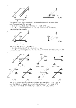
![51
Deflection of Grids due to Combined Flexural and Torsional Deformations
Grids are 2-dimensional (coplanar) structures with one deflection and two rotations at each node.
If the structure is in the x-z plane, the deflection is out-of-plane (along the y axis) while the rotations are
about two in-plane axes (x and z axis). Grids are loaded perpendicular to the structural plane and have three
forces per member; i.e., shear force, bending moment and torsion.
Example
EI = 40 103
k-ft2
GJ = 30 103
k-ft2
Top View Isometric View
150
50
50 50
10
5
5
1
A,v = (m1 m0/EI) dS + (t1 t0/GJ) dS
= {[5 5 (–50)/3] + 5 [5 (–250)+10 (–350)]/6}/(40 103
) +{10 (–5) (–50)}/(30 103
)
= –109.38 10–3
+ 83.33 10–3
= –26.05 10–3
ft
10
5
5
1
C,v = {[5 5 (–50)/3]+[5 5 (–50)/3]+5 [5 (–250)+10 (–350)]/6}/(40 103
) + {10 (5) (–50)}/(30 103
)
= –120.80 10–3
– 83.33 10–3
= –204.13 10–3
ft
5
EE
Calculate A,v and C,v if
10 k
10 k
A
D
10 k
10 k
D
A B CB C
5
5
55
5
Calculation of A,v
Calculation of C,v
m1 ( ) t1 ( )
m1 ( ) t1 ( )
m0 (k ) t0 (k )](https://image.slidesharecdn.com/structuralengineeringii1-160123221338/85/Structural-engineering-ii-51-320.jpg)
![53
Deflection of Grids using Method of Virtual Work
1.
D = [(−50)(5)5/3 + {2(−62.5) + (−150)}(10)(10)/6]/(40 103
) + [(−50)(5)10]/(30 103
)
= −0.125 −0.0833 = −0.2083 ft
2.
E = [(−50)(5)5/3 + (−50)(5)5/3 + {(−50) (25) + (−250) (35)}(10)/6]/(40 103
) + [(50)(−5)5]/(30 103
)
= −0.4375 −0.0417 = −0.4792 ft
10
50
150
62.5
m0 (k-ft)
50
t0 (k-ft) m1 (ft) t1 (ft)
55
A
B C D
For D
50
250
m0 (k-ft)
50
t0 (k-ft) m1 (ft) t1 (ft)
5
A
B C
D
For E
E
50
5
15
5
5](https://image.slidesharecdn.com/structuralengineeringii1-160123221338/85/Structural-engineering-ii-53-320.jpg)
![54
3.
D = [(−100)(10)10/3 + (−50)(5)5/3 + {(−50) (20) + (−150) (25)}(5)/6]/(40 103
) +
[(100 + 150)(−10)5]/(30 103
)
= −0.1927 −0.4167 = −0.6094 ft
4.
D = [(12.5)(−2.5) 5/3 2]/(40 103
)
= −26.04 10-3
ft
A
B
C
D
10
100
150
50
m0 (k-ft)
100
t0 (k-ft) m1 (ft) t1 (ft)
10
10
A
B
C
For D
D
E
150
m0 (k-ft) t0 (k-ft) m1 (ft) t1 (ft)
For C
12.5
12.5
−2.5
5](https://image.slidesharecdn.com/structuralengineeringii1-160123221338/85/Structural-engineering-ii-54-320.jpg)
![55
Flexibility Method for Grids (Combined Flexural and Torsional Deformations)
Grids are 2-dimensional (coplanar) structures with one deflection and two rotations at each node.
If the structure is in the x-z plane, the deflection is out-of-plane (along the y axis) while the rotations are
about two in-plane axes (x and z axis).
Grids are loaded perpendicular to the structural plane and have three forces per member; i.e., shear force,
bending moment and torsion.
Example
E
E
5 EI = 40 103
k-ft2
10 k
GJ = 30 103
k-ft2
dosi = 3 3 + 4 – 3 4 = 1 D
5 10 k
A B C A B C
5 5
Top View Isometric View
10 k
150
10 k 50
1,0
50 50
Case 0 m0 (k ) t0 (k )
10
5
1,1
5
1 5
Case 1 m1 ( ) t1 ( )
1,0 = (m1 m0/EI) dS + (t1 t0/GJ) dS
= {[5 5 (–50)/3] + 5 [5 (–250)+10 (–350)]/6}/(40 103
) +{10 (–5) (–50)}/(30 103
)
= –109.38 10–3
+ 83.33 10–3
= –26.05 10–3
ft
1,1 = (m1 m1/EI) dS + (t1 t1/GJ) dS
={5 (5 5)/3+10 (10 10)/3}/(40 103
) +{10 (–5) (–5)}/(30 103
)
= 9.38 10–3
+ 8.33 10–3
= 17.71 10–3
ft/k
VA = 26.05 10–3
/17.71 10–3
= 1.47 k
D](https://image.slidesharecdn.com/structuralengineeringii1-160123221338/85/Structural-engineering-ii-55-320.jpg)

The document discusses the analysis of portal frame structures and multi-storied buildings using the portal and cantilever methods. It emphasizes the importance of understanding the degree of statical indeterminacy and making appropriate assumptions for accurate analysis of loads and moments in the structures. Additionally, examples are provided to illustrate the application of these methods in calculating shear forces, bending moments, and axial forces.