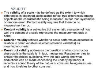
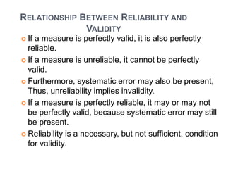
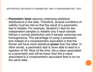
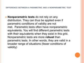
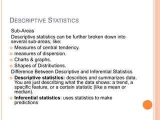
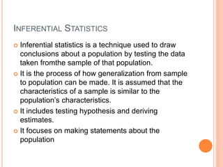
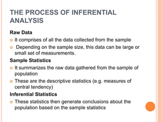
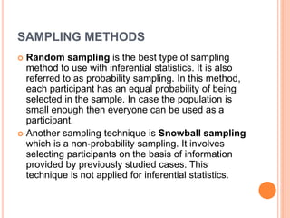
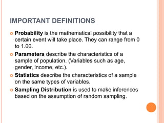
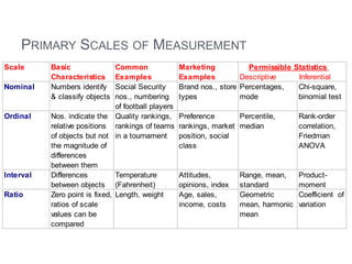
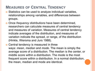
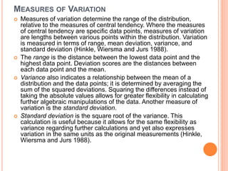
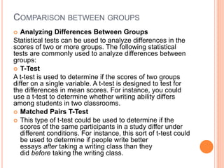
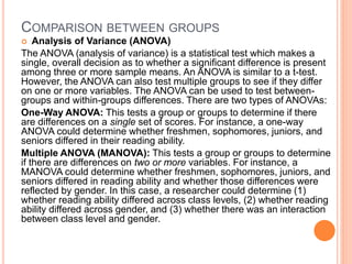
SlideShare a Scribd company logo
BASIC CONCEPTS OF
INFERENTIAL STATISTICS
DR. QAISAR ABBAS
WHAT IS STATISTICS?
It is the branch of scientific methodology. It deals with
the collection, classification, description and
interpretation of data obtained by conduct of
surveys and experiment. Its essential purpose is to
describe and draw inferences about the numerical
properties of population.
DESCRIPTIVE STATISTICS
 Descriptive statistics are one of the fundamental
“must knows” with any set of data. It gives you a
general idea of trends in your data including:
 The mean, mode, median and range.
 Variance and standard deviation.
 Skewness
 Count, maximum and minimum.
DESCRIPTIVE STATISTICS
 Descriptive statistics is useful because it allows you
to take a large amount of data and summarize it.
For example, let’s say you had data on the incomes
of one million people. No one is going to want to
read a million pieces of data; if they did, they
wouldn’t be able to glean any useful information
from it. On the other hand, if you summarize it, it
becomes useful: an average wage, or a median
income, is much easier to understand than reams
of data.
DESCRIPTIVE STATISTICS
Sub-Areas
Descriptive statistics can be further broken down into
several sub-areas, like:
 Measures of central tendency.
 measures of dispersion.
 Charts & graphs.
 Shapes of Distributions.
Difference Between Descriptive and Inferential Statistics
 Descriptive statistics: describes and summarizes data.
You are just describing what the data shows: a trend, a
specific feature, or a certain statistic (like a mean or
median).
 Inferential statistics: uses statistics to make
predictions
INFERENTIAL STATISTICS
 Inferential statistics is a technique used to draw
conclusions about a population by testing the data
taken fromthe sample of that population.
 It is the process of how generalization from sample
to population can be made. It is assumed that the
characteristics of a sample is similar to the
population’s characteristics.
 It includes testing hypothesis and deriving
estimates.
 It focuses on making statements about the
population
THE PROCESS OF INFERENTIAL
ANALYSIS
Raw Data
 It comprises of all the data collected from the sample
 Depending on the sample size, this data can be large or
small set of measurements.
Sample Statistics
 It summarizes the raw data gathered from the sample of
population
 These are the descriptive statistics (e.g. measures of
central tendency)
Inferential Statistics
 These statistics then generate conclusions about the
population based on the sample statistics
SAMPLING METHODS
 Random sampling is the best type of sampling
method to use with inferential statistics. It is also
referred to as probability sampling. In this method,
each participant has an equal probability of being
selected in the sample. In case the population is
small enough then everyone can be used as a
participant.
 Another sampling technique is Snowball sampling
which is a non-probability sampling. It involves
selecting participants on the basis of information
provided by previously studied cases. This
technique is not applied for inferential statistics.
IMPORTANT DEFINITIONS
 Probability is the mathematical possibility that a
certain event will take place. They can range from 0
to 1.00.
 Parameters describe the characteristics of a
sample of population. (Variables such as age,
gender, income, etc.).
 Statistics describe the characteristics of a sample
on the same types of variables.
 Sampling Distribution is used to make inferences
based on the assumption of random sampling.
SAMPLING ERROR CONCEPTS
 Sampling Error: Inferential statistics takes
sampling error (random error) into account. It is the
degree to which a sample differs on a key variable
from the population.
 Confidence Level: The number of times out of 100
that the true value will fall within the confidence
interval.
 Confidence Interval: A calculated range for the
true value, based on the relative sizes of the
sample and the population
 Sampling error describes the difference between
sample statistics and population parameters
SAMPLING DISTRIBUTION CONCEPTS
 The variables of a sample taken from the
population should be the same for the population
also.
 Due to sampling error, the sample mean can be
varied.
 The amount of this variation in the sample mean is
referred to as standard error
 Standard error decreases as the sample size
increases.
TYPES OF HYPOTHESES
 Alternative hypothesis: It specifies expected
relationship between two or more variables. It may
be symbolized by H1 or Ha.
 Null hypothesis: It is the statement that says there
is no real relationship between the variables
described in the alternative hypothesis
 In inferential statistics, the hypothesis that is
actually tested is the null hypothesis. Therefore, it is
essential to prove that the null hypothesis is not
valid and alternative hypothesis is true and should
be accepted.
HYPOTHESIS TESTING PROCESS
 State the research hypothesis
 State the null hypothesis
 Choose a level of statistical significance
 Select and compute the test statistic
 Make a decision regarding whether to accept or
reject the null hypothesis
EXAMPLES
Let’s say you have some sample data about a potential new
cancer drug. You could use descriptive statistics to describe
your sample, including:
 Sample mean, Sample standard deviation, Making a bar
chart or boxplot
 Describing the shape of the sample probability distribution
A bar graph is one way to summarize data in descriptive statistics
INFERENTIAL STATISTICS
But in inferential statistics you take that sample data from a
small number of people and try to determine if the data can
predict whether the drug will work for everyone (i.e. the
population). There are various ways you can do this, from
calculating a z-score (z-scores are a way to show where your
data would lie in a normal distribution to post-hoc (advanced)
testing.
INFERENTIAL STATISTICS
Inferential statistics use statistical models to help you compare
your sample data to other samples or to previous research.
Most research uses statistical models called the Generalized
Linear model and include Student’s t-tests, ANOVA (Analysis of
Variance), regression analysis and various other models that
result in straight-line (“linear”) probabilities and results.
WHAT IS POPULATION?
 A population is a group to which a researcher would
like the results of a study to be generalizable
 A defined population has at least one characteristic
that differentiates it from other groups
 The population that the researcher would ideally
like to generalize results to is referred to as the
target population; the population that the researcher
realistically selects from is referred as the
accessible or available population
WHAT IS SAMPLING?
 Sampling is the process of selecting a number of
individuals for a study in such a way that the
individuals represent the larger group from which
they were selected
 The purpose of sampling is to use a sample to gain
information about a population
PARAMETERS AND ESTIMATES
 A parameter is a property descriptive of the
population.
 The term estimate refers to a property of a sample
drawn at random from a population.
EXAMPLE
A sample of 1000 adult male Pakistani of a given age
range is drawn from the total population. The height
of the members of the sample measured, and the
mean value, 68.972 inches obtained. This value is
estimate of the population parameter.
VARIABLES AND THEIR CLASSIFICATIONS
The term variable refers to a property whereby the
members of a group or set differ one from another.
The members of the group may be individuals and
may be found to differ in sex, age, eye color,
intelligence, reaction time to a stimulus, attitude
towards political issues and many other ways. Such
properties are called variables.
CONSTANT
The term constant refers to a property whereby the
members of a group do not differ one from another.
It is a variable which does not vary from one
member of a group to another or with in a
particulars set of defined conditions.
4 BROAD CLASSES OF VARIABLES/SCALES
 Nominal scale
 Ordinal scale
 Interval scale
 Ratio scale
7 38
PRIMARY SCALES OF MEASUREMENT
Scale
Nominal Numbers
Assigned
to Runners
Ordinal Rank Order
of Winners
Interval Performance
Rating on a
0 to 10 Scale
Ratio Time to
Finish, in
Seconds
Third
place
Second
place
First
place
Finish
Finish
8.2 9.1 9.6
15.2 14.1 13.4
NOMINAL SCALE
 The numbers serve only as labels or tags for
identifying and classifying objects.
 When used for identification, there is a strict one-to-
one correspondence between the numbers and the
objects.
 The numbers do not reflect the amount of the
characteristic possessed by the objects.
 The only permissible operation on the numbers in a
nominal scale is counting.
 Social security number, hockey players number.
marketing research respondents, brands, attributes,
stores and other objects
ORDINAL SCALE
 A ranking scale in which numbers are assigned to
objects to indicate the relative extent to which the
objects possess some characteristic.
 Can determine whether an object has more or less of a
characteristic than some other object, but not how
much more or less.
 Any series of numbers can be assigned that preserves
the ordered relationships between the objects. So
relative position of objects not the magnitude of
difference between the objects.
 In addition to the counting operation allowable for
nominal scale data, ordinal scales permit the use of
statistics based on percentile, quartile, median.
 Possess description and order, not distance or origin
INTERVAL SCALE
 Numerically equal distances on the scale represent
equal values in the characteristic being measured.
 It permits comparison of the differences between
objects.
 The difference between 1 & 2 is same as between
2 & 3
 The location of the zero point is not fixed. Both the
zero point and the units of measurement are
arbitrary.
 Everyday temperature scale. Attitudinal data
obtained on rating scales.
 Do not possess origin characteristics (zero and
exact measurement)
RATIO SCALE
 The highest scale that allows to identify objects,
rank order of objects, and compare intervals or
differences. It is also meaningful to compute ratios
of scale values
 Possesses all the properties of the nominal, ordinal,
and interval scales. It has an absolute zero point.
 Height, weight, age, money. Sales, costs, market
share and number of customers are variables
measured on a ratio scale
 All statistical techniques can be applied to ratio
data.
ILLUSTRATION OF PRIMARY SCALES OF
MEASUREMENT
Nominal Ordinal Ratio
Scale Scale Scale
Preference $ spent last
No. Store Rankings 3 months
1. Lord & Taylor
2. Macy’s
3. Kmart
4. Rich’s
5. J.C. Penney
6. Neiman Marcus
7. Target
8. Saks Fifth Avenue
9. Sears
10.Wal-Mart
Interval
Scale
Preference
Ratings
1-7 11-17
7 79 5 15 0
2 25 7 17 200
8 82 4 14 0
3 30 6 16 100
1 10 7 17 250
5 53 5 15 35
9 95 4 14 0
6 61 5 15 100
4 45 6 16 0
10 115 2 12 10
PRIMARY SCALES OF MEASUREMENT
Scale Basic
Characteristics
Common
Examples
Marketing
Examples
Nominal Numbers identify
& classify objects
Social Security
nos., numbering
of football players
Brand nos., store
types
Percentages,
mode
Chi-square,
binomial test
Ordinal Nos. indicate the
relative positions
of objects but not
the magnitude of
differences
between them
Quality rankings,
rankings of teams
in a tournament
Preference
rankings, market
position, social
class
Percentile,
median
Rank-order
correlation,
Friedman
ANOVA
Ratio Zero point is fixed,
ratios of scale
values can be
compared
Length, weight Age, sales,
income, costs
Geometric
mean, harmonic
mean
Coefficient of
variation
Permissible Statistics
Descriptive Inferential
Interval Differences
between objects
Temperature
(Fahrenheit)
Attitudes,
opinions, index
Range, mean,
standard
Product-
moment
SCALE EVALUATION
Discriminant NomologicalConvergent
Test/
Retest
Alternative
Forms
Internal
Consistency
Content Criterion Construct
GeneralizabilityReliability Validity
Scale Evaluation
RELIABILITY
 Reliability can be defined as the extent to which
measures are free from random error, the measure is
perfectly reliable.
 In test-retest reliability, respondents are
administered identical sets of scale items at two
different times and the degree of similarity between
the two measurements is determined.
 In alternative-forms reliability, two equivalent forms
of the scale are constructed and the same
respondents are measured at two different times, with
a different form being used each time.
RELIABILITY
 Internal consistency reliability determines the
extent to which different parts of a summated scale
are consistent in what they indicate about the
characteristic being measured.
 In split-half reliability, the items on the scale are
divided into two halves and the resulting half scores
are correlated.
 The coefficient alpha, or Cronbach's alpha, is the
average of all possible split-half coefficients
resulting from different ways of splitting the scale
items. This coefficient varies from 0 to 1, and a
value of 0.6 or less generally indicates
unsatisfactory internal consistency reliability.
VALIDITY
 The validity of a scale may be defined as the extent to which
differences in observed scale scores reflect true differences among
objects on the characteristic being measured, rather than systematic
or random error. Perfect validity requires that there be no
measurement error.
 Content validity is a subjective but systematic evaluation of how
well the content of a scale represents the measurement task at
hand.
 Criterion validity reflects whether a scale performs as expected in
relation to other variables selected (criterion variables) as
meaningful criteria.
 Construct validity addresses the question of what construct or
characteristic the scale is, in fact, measuring. Researcher tries to
answer theoretical questions, why the sale works and what
deductions can be made concerning the underlying theory. It
requires a sound theory of the nature of construct being measures
and how it relates to other construct
RELATIONSHIP BETWEEN RELIABILITY AND
VALIDITY
 If a measure is perfectly valid, it is also perfectly
reliable.
 If a measure is unreliable, it cannot be perfectly
valid.
 Furthermore, systematic error may also be present,
Thus, unreliability implies invalidity.
 If a measure is perfectly reliable, it may or may not
be perfectly valid, because systematic error may still
be present.
 Reliability is a necessary, but not sufficient, condition
for validity.
DIFFERENCE BETWEEN A PARAMETRIC AND A NONPARAMETRIC TEST
 Parametric tests assume underlying statistical
distributions in the data. Therefore, several conditions of
validity must be met so that the result of a parametric
test is reliable. For example, Student’s t-test for two
independent samples is reliable only if each sample
follows a normal distribution and if sample variances are
homogeneous. The advantage of using a parametric
test instead of a nonparametric equivalent is that the
former will have more statistical power than the latter. In
other words, a parametric test is more able to lead to a
rejection of H0. Most of the time, the p-value associated
to a parametric test will be lower than the p-value
associated to a nonparametric equivalent that is run on
the same data.
DIFFERENCE BETWEEN A PARAMETRIC AND A NONPARAMETRIC TEST
 Nonparametric tests do not rely on any
distribution. They can thus be applied even if
parametric conditions of validity are not
met. Parametric tests often have nonparametric
equivalents. You will find different parametric tests
with their equivalents when they exist in this grid.
Nonparametric tests are more robust than
parametric tests. In other words, they are valid in a
broader range of situations (fewer conditions of
validity)
TYPES OF ERROR IN STATISTICS
 Type I Errors occur when we reject a null hypothesis
that is actually true; the probability of this occurring is
denoted by alpha (a).
 Type II Errors are when we accept a null hypothesis
that is actually false; its probability is called beta (b).
 As you can see from the below table, the other two
options are to accept a true null hypothesis, or to reject
a false null hypothesis. Both of these are correct, though
one is far more exciting than the other (and probably
easier to get published).
CLASSIFICATION OF SAMPLING TECHNIQUES
Sampling Techniques
Nonprobability
Sampling Techniques
Probability
Sampling Techniques
Convenience
Sampling
Judgmental
Sampling
Quota
Sampling
Snowball
Sampling
Systematic
Sampling
Stratified
Sampling
Cluster
Sampling
Other Sampling
Techniques
Simple Random
Sampling
No probability sampling relies on personal judgment of the
researcher rather than chance to select sample elements.
The researcher can arbitrary or consciously decide what
elements to include in the sample and may yield good
estimates of the population characteristics. The estimates
obtained are not statistically projectable to the population.
Probability sampling is a procedure in which each element of
the population has a fixed probabilistic chance of being
selected for the sample. Sampling units are selected by
chance. It requires a precise definition of the target
population and general specification of the sampling frame.
Confidence intervals which contain the true population value
with a given level of certainty, can be calculated. This allows
researcher to make inferences and projections about the
target population, from which sample was drawn.
NO PROBABILITY: CONVENIENCE
SAMPLING
Convenience sampling attempts to obtain a
sample of convenient elements. Often,
respondents are selected because they happen to
be in the right place at the right time.
 use of students, and members of social
organizations
 mall intercept interviews without qualifying the
respondents
 department stores using charge account lists
 “people on the street” interviews
JUDGMENTAL SAMPLING
Judgmental sampling is a form of convenience
sampling in which the population elements are
selected based on the judgment of the researcher.
 test markets
 purchase engineers selected in industrial
marketing research
 bellwether precincts selected in voting behavior
research
 expert witnesses used in court
QUOTA SAMPLING
Quota sampling may be viewed as two-stage restricted judgmental
sampling.
 The first stage consists of developing control categories, or quotas, of
population elements.
 In the second stage, sample elements are selected based on
convenience or judgment.
Population Sample
composition composition
Control
Characteristic Percentage Percentage Number
Sex
Male 48 48 480
Female 52 52 520
____ ____ ____
100 100 1000
SNOWBALL SAMPLING
In snowball sampling, an initial group of
respondents is selected, usually at random.
 After being interviewed, these respondents are
asked to identify others who belong to the target
population of interest.
 Subsequent respondents are selected based on
the referrals.
PROBABILITY: SIMPLE RANDOM SAMPLING
 Each element in the population has a known
and equal probability of selection.
 Each possible sample of a given size (n)
has a known and equal probability of being
the sample actually selected.
 This implies that every element is selected
independently of every other element.
PROCEDURES FOR DRAWING PROBABILITY
SAMPLESSimple
Random
Sampling
1. Select a suitable sampling frame
2. Each element is assigned a number from 1 to N
(pop. size)
3. Generate n (sample size) different random numbers
between 1 and N
4. The numbers generated denote the elements that
should be included in the sample
SYSTEMATIC SAMPLING
 The sample is chosen by selecting a random starting point and
then picking every kith element in succession from the sampling
frame.
 The sampling interval, i, is determined by dividing the population
size N by the sample size n and rounding to the nearest integer.
 When the ordering of the elements is related to the characteristic
of interest, systematic sampling increases the representativeness
of the sample.
 If the ordering of the elements produces a cyclical pattern,
systematic sampling may decrease the representativeness of the
sample.
For example, there are 100,000 elements in the population and a
sample of 1,000 is desired. In this case the sampling interval, i, is
100. A random number between 1 and 100 is selected. If, for
example, this number is 23, the sample consists of elements 23,
123, 223, 323, 423, 523, and so on.
PROCEDURES FOR DRAWING
PROBABILITY SAMPLES
Systematic
Sampling
1. Select a suitable sampling frame
2. Each element is assigned a number from 1 to N (pop. size)
3. Determine the sampling interval i:i=N/n. If i is a fraction,
round to the nearest integer
4. Select a random number, r, between 1 and i, as explained in
simple random sampling
5. The elements with the following numbers will comprise the
systematic random sample: r, r+i,r+2i,r+3i,r+4i,...,r+(n-1)i
STRATIFIED SAMPLING
 A two-step process in which the population is
partitioned into subpopulations, or strata.
 The strata should be mutually exclusive and
collectively exhaustive in that every population
element should be assigned to one and only one
stratum and no population elements should be
omitted.
 Next, elements are selected from each stratum by a
random procedure, usually SRS.
 A major objective of stratified sampling is to
increase precision without increasing cost.
1. Select a suitable frame
2. Select the stratification variable(s) and the number of strata, H
3. Divide the entire population into H strata. Based on the
classification variable, each element of the population is assigned
to one of the H strata
4. In each stratum, number the elements from 1 to Nh (the pop.
size of stratum h)
5. Determine the sample size of each stratum, nh, based on
proportionate or disproportionate stratified sampling, where
6. In each stratum, select a simple random sample of size nh
PROCEDURES FOR DRAWING
PROBABILITY SAMPLES
nh = n
h=1
H
Stratified
Sampling
CLUSTER SAMPLING
 The target population is first divided into mutually exclusive and
collectively exhaustive subpopulations, or clusters.
 Then a random sample of clusters is selected, based on a
probability sampling technique such as SRS.
 For each selected cluster, either all the elements are included in the
sample (one-stage) or a sample of elements is drawn
probabilistically (two-stage).
 Elements within a cluster should be as heterogeneous (mixed) as
possible, but clusters themselves should be as homogeneous
(uniform) as possible. Ideally, each cluster should be a small-scale
representation of the population.
 In probability proportionate to size sampling, the clusters are
sampled with probability proportional to size. In the second stage,
the probability of selecting a sampling unit in a selected cluster
varies inversely with the size of the cluster.
PROCEDURES FOR DRAWING
PROBABILITY SAMPLES
Cluster
Sampling
1. Assign a number from 1 to N to each element in the population
2. Divide the population into C clusters of which c will be included in
the sample
3. Calculate the sampling interval i, i=N/c (round to nearest integer)
4. Select a random number r between 1 and i, as explained in simple
random sampling
5. Identify elements with the following numbers:
r,r+i,r+2i,... r+(c-1)i
6. Select the clusters that contain the identified elements
7. Select sampling units within each selected cluster based on SRS
or systematic sampling
8. Remove clusters exceeding sampling interval i. Calculate new
population size N*, number of clusters to be selected C*= C-1,
and new sampling interval i*.
PROCEDURES FOR DRAWING PROBABILITY
SAMPLES
Repeat the process until each of the remaining
clusters has a population less than the
sampling interval. If b clusters have been
selected with certainty, select the remaining c-
b clusters according to steps 1 through 7. The
fraction of units to be sampled with certainty is
the overall sampling fraction = n/N. Thus, for
clusters selected with certainty, we would
select ns=(n/N)(N1+N2+...+Nb) units. The units
selected from clusters selected under PPS
sampling will therefore be n*=n- ns.
Cluster
Sampling
Non probability Sampling
Technique Strengths Weaknesses
Convenience Least expensive, least time-
consuming, most convenient
Selection bias, sample not representative, not
recommended for descriptive or causal research
Judgmental Low cost, convenient, not time-
consuming
Does not allow generalization, subjective
Quota Sample can be controlled for
certain characteristics
Selection bias, no assurance of representativeness
Snowball Can estimate rare
characteristics
Time-consuming
Probability Sampling
Simple
random (SRS)
Easily understood, results
projectable
Difficult to construct sampling frame, expensive, lower
precision, no assurance of representativeness
Systematic Can increase repre…tiveness,
easier to implement than SRS,
sampling frame not necessary
Can decrease repre..iveness
if there are cyclical patterns
Stratified Includes all important
subpopulations, precision
Difficult to select relevant stratification variables, not
feasible to stratify on many variables, expensive
Cluster Easy to implement, Cost -
effective
Imprecise, Difficult to compute and interpret results
CHOOSING NONPROBABILITY VS. PROBABILITY
SAMPLING
Conditions Favoring the Use of
Factors Nonprobability
sampling
Probability
sampling
Nature of research Exploratory Conclusive
Relative magnitude of sampling
and nonsampling errors
Nonsampling
errors are
larger
Sampling
errors are
larger
Variability in the population Homogeneous
(low)
Heterogeneous
(high)
Statistical considerations Unfavorable Favorable
Operational considerations Favorable Unfavorable
FINDING MEAN, MEDIAN AND MODE
 Mean, median, and mode are three kinds of "averages". There
are many "averages" in statistics, but these are, I think, the
three most common, and are certainly the three you are most
likely to encounter in your statistics.
 The "mean" is the "average" you're used to, where you add up
all the numbers and then divide by the number of numbers.
 The "median" is the "middle" value in the list of numbers. To
find the median, your numbers have to be listed in numerical
order from smallest to largest, so you may have to rewrite your
list before you can find the median.
 The "mode" is the value that occurs most often. If no number
in the list is repeated, then there is no mode for the list.
 The "range" of a list a numbers is just the difference between
the largest and smallest values.
MEAN FORMULA
FINDING MEAN, MEDIAN AND MODE
Find the mean, median, mode, and range for the following list of values:
1, 2, 4, 7
The mean is the usual average:
(1 + 2 + 4 + 7) ÷ 4
= 14 ÷ 4 = 3.5
=3.5 is Mean
The median is the middle number. In this example, the numbers are already listed in
numerical order, so I don't have to rewrite the list. But there is no "middle" number,
because there are an even number of numbers. Because of this, the median of the
list will be the mean (that is, the usual average) of the middle two values within the
list. The middle two numbers are 2 and 4, so:
(2 + 4) ÷ 2 = 6 ÷ 2 = 3 (So the median of this list is 3)

The mode is the number that is repeated most often, but all the numbers in this
list appear only once, so there is no mode.
 The largest value in the list is 7, the smallest is 1, and their difference is 6, so the
range is 6.
 mean: 3.5, median: 3, mode: none, range: 6
EXAMPLE 2
 Find the mean, median, mode, and range for the following
list of values:
13, 18, 13, 14, 13, 16, 14, 21, 13
The mean is the usual average, so I'll add and then divide:
(13 + 18 + 13 + 14 + 13 + 16 + 14 + 21 + 13) ÷ 9 = 15
The median is the middle value, so first I'll have to rewrite the list
in numerical order:
13, 13, 13, 13, 14, 14, 16, 18, 21
There are nine numbers in the list, so the middle one will be
the (9 + 1) ÷ 2 = 10 ÷ 2 = 5th number:
13, 13, 13, 13, 14, 14, 16, 18, 21
The mode is the number that is repeated more often than any
other, so 13 is the mode.
The largest value in the list is 21, and the smallest is 13, so the
range is 21 – 13 = 8.
Thus
mean: 15, median: 14, mode: 13, range: 8
CALCULATION OF MEAN FROM GROUP DATA
ANALYZING INDIVIDUAL VARIABLES
 The statistical procedures used to analyze a single variable
describing a group (such as a population or representative
sample) involve measures of central tendency and measures
of variation. To explore these measures, a researcher first
needs to consider the distribution, or range of values of a
particular variable in a population or sample. Normal
distribution occurs if the distribution of a population is
completely normal. When graphed, this type of distribution will
look like a bell curve; it is symmetrical and most of the scores
cluster toward the middle.
 Skewed Distribution simply means the distribution of a
population is not normal. The scores might cluster toward the
right or the left side of the curve, for instance. Or there might
be two or more clusters of scores, so that the distribution
looks like a series of hills.
MEASURES OF CENTRAL TENDENCY
 Statistics can be used to analyze individual variables,
relationships among variables, and differences between
groups.
 Once frequency distributions have been determined,
researchers can calculate measures of central tendency
and measures of variation. Measures of central tendency
indicate averages of the distribution, and measures of
variation indicate the spread, or range, of the distribution
(Hinkle, Wiersma and Jurs 1988).
 Central tendency is measured in three
ways: mean, median and mode. The mean is simply the
average score of a distribution. The median is the center, or
middle score within a distribution. The mode is the most
frequent score within a distribution. In a normal distribution,
the mean, median and mode are identical.
MEASURES OF VARIATION
 Measures of variation determine the range of the distribution,
relative to the measures of central tendency. Where the measures
of central tendency are specific data points, measures of variation
are lengths between various points within the distribution. Variation
is measured in terms of range, mean deviation, variance, and
standard deviation (Hinkle, Wiersma and Jurs 1988).
 The range is the distance between the lowest data point and the
highest data point. Deviation scores are the distances between
each data point and the mean.
 Variance also indicates a relationship between the mean of a
distribution and the data points; it is determined by averaging the
sum of the squared deviations. Squaring the differences instead of
taking the absolute values allows for greater flexibility in calculating
further algebraic manipulations of the data. Another measure of
variation is the standard deviation.
 Standard deviation is the square root of the variance. This
calculation is useful because it allows for the same flexibility as
variance regarding further calculations and yet also expresses
variation in the same units as the original measurements (Hinkle,
Wiersma and Jurs 1988).
COMPARISON BETWEEN GROUPS
 Analyzing Differences Between Groups
Statistical tests can be used to analyze differences in the
scores of two or more groups. The following statistical
tests are commonly used to analyze differences between
groups:
 T-Test
A t-test is used to determine if the scores of two groups
differ on a single variable. A t-test is designed to test for
the differences in mean scores. For instance, you could
use a t-test to determine whether writing ability differs
among students in two classrooms.
 Matched Pairs T-Test
 This type of t-test could be used to determine if the
scores of the same participants in a study differ under
different conditions. For instance, this sort of t-test could
be used to determine if people write better
essays after taking a writing class than they
did before taking the writing class.
COMPARISON BETWEEN GROUPS
 Analysis of Variance (ANOVA)
The ANOVA (analysis of variance) is a statistical test which makes a
single, overall decision as to whether a significant difference is present
among three or more sample means. An ANOVA is similar to a t-test.
However, the ANOVA can also test multiple groups to see if they differ
on one or more variables. The ANOVA can be used to test between-
groups and within-groups differences. There are two types of ANOVAs:
One-Way ANOVA: This tests a group or groups to determine if there
are differences on a single set of scores. For instance, a one-way
ANOVA could determine whether freshmen, sophomores, juniors, and
seniors differed in their reading ability.
Multiple ANOVA (MANOVA): This tests a group or groups to determine
if there are differences on two or more variables. For instance, a
MANOVA could determine whether freshmen, sophomores, juniors, and
seniors differed in reading ability and whether those differences were
reflected by gender. In this case, a researcher could determine (1)
whether reading ability differed across class levels, (2) whether reading
ability differed across gender, and (3) whether there was an interaction
between class level and gender.
COMPARISON BETWEEN GROUPS
 Analysis of Variance (ANOVA)
 The two-way ANOVA compares the mean differences
between groups that have been split on two independent
variables (called factors). The primary purpose of a two-
way ANOVA is to understand if there is an interaction
between the two independent variables on the dependent
variable. For example, you could use a two-way ANOVA
to understand whether there is an interaction between
gender and educational level on test anxiety amongst
university students, where gender (males/females) and
education level (undergraduate/postgraduate) are your
independent variables, and test anxiety is your
dependent variable.
COMPARISON BETWEEN GROUPS
 Analyzing Relationships Among Variables
Statistical relationships between variables rely on notions of
correlation and regression. These two concepts aim to describe
the ways in which variables relate to one another:
Correlation
Correlation tests are used to determine how strongly the scores
of two variables are associated or correlated with each other. A
researcher might want to know, for instance, whether a
correlation exists between students' writing placement
examination scores and their scores on a standardized test such
as the ACT or SAT. Correlation is measured using values
between +1.0 and -1.0. Correlations close to 0 indicate little or
no relationship between two variables, while correlations close to
+1.0 (or -1.0) indicate strong positive (or negative) relationships
(Hayes et al. 554).
COMPARISON BETWEEN GROUPS
Correlation
 Correlation denotes positive or negative association between
variables in a study. Two variables are positively
associated when larger values of one tend to be accompanied
by larger values of the other. The variables are negatively
associated when larger values of one tend to be accompanied
by smaller values of the other (Moore 208).
 An example of a strong positive correlation would be the
correlation between age and job experience. Typically, the
longer people are alive, the more job experience they might
have.
 An example of a strong negative relationship might occur
between the strength of people's party affiliations and their
willingness to vote for a candidate from different parties. In
many elections, Democrats are unlikely to vote for
Republicans, and vice versa.
COMPARISON BETWEEN GROUPS
Regression
Regression analysis attempts to determine the best "fit" between two or
more variables. The independent variable in a regression analysis is a
continuous variable, and thus allows you to determine how one or more
independent variables predict the values of a dependent variable.
Simple Linear Regression is the simplest form of regression. Like a
correlation, it determines the extent to which one independent variables
predicts a dependent variable. You can think of a simple linear regression
as a correlation line. Regression analysis provides you with more
information than correlation does, however. It tells you how well the line
"fits" the data. That is, it tells you how closely the line comes to all of your
data points. The line in the figure indicates the regression line drawn to find
the best fit among a set of data points. Each dot represents a person and
the axes indicate the amount of job experience and the age of that person.
The dotted lines indicate the distance from the regression line. A smaller
total distance indicates a better fit. Some of the information provided in a
regression analysis, as a result, indicates the slope of the regression line,
the R value (or correlation), and the strength of the fit (an indication of the
extent to which the line can account for variations among the data points).
COMPARISON BETWEEN GROUPS
Regression
Multiple Linear Regression allows one to determine how
well multiple independent variables predict the value of a
dependent variable. A researcher might examine, for
instance, how well age and experience predict a person's
salary. The interesting thing here is that one would no
longer be dealing with a regression "line." Instead, since
the study deals with three dimensions (age, experience,
and salary), it would be dealing with a plane, that is, with a
two-dimensional figure. If a fourth variable was added to
the equations, one would be dealing with a three-
dimensional figure, and so on.
COMPARISON BETWEEN GROUPS
factorial analysis of variance
 A factorial ANOVA is an Analysis of Variance test with more
than one independent variable, or “factor“. It can also refer to
more than one Level of Independent Variable. For example,
an experiment with a treatment group and a control group has
one factor (the treatment) but two levels (the treatment and the
control). The terms “two-way” and “three-way” refer to the
number of factors or the number of levels in your test. Four-
way ANOVA and above are rarely used because the results of
the test are complex and difficult to interpret.
 Factorial ANOVA is an efficient way of conducting a test.
Instead of performing a series of experiments where you test
one independent variable against one dependent variable, you
can test all independent variables at the same time.
COMPARISON BETWEEN GROUPS
Factors affecting correlation
Pearson’s correlation coefficient is the test statistics that
measures the statistical relationship, or association, between two
continuous variables. It is known as the best method of
measuring the association between variables of interest because
it is based on the method of covariance. It gives information
about the magnitude of the association, or correlation, as well as
the direction of the relationship.
The authors describe and illustrate 6 factors that affect the size
of a Pearson correlation: (a) the amount of variability in the
data,
(b) differences in the shapes of the 2 distributions,
(c) lack of linearity,
(d) the presence of 1 or more "outliers,"
(e) characteristics of the sample, and
(f) measurement error.
COMPARISON BETWEEN GROUPS
Degree of correlation:
 Perfect: If the value is near ± 1, then it said to be a
perfect correlation: as one variable increases, the other
variable tends to also increase (if positive) or decrease (if
negative).
 High degree: If the coefficient value lies between ± 0.50
and ± 1, then it is said to be a strong correlation.
 Moderate degree: If the value lies between ± 0.30 and ±
0.49, then it is said to be a medium correlation.
 Low degree: When the value lies below + .29, then it is
said to be a small correlation.
 No correlation: When the value is zero.
COMPARISON BETWEEN GROUPS
Multiple correlation:
In statistics, the coefficient of multiple correlation is a measure of how
well a given variable can be predicted using a linear function of a set of
other variables. It is the correlation between the variable's values and
the best predictions that can be computed linearly from the predictive
variables.
 The coefficient of multiple correlation takes values between .00 and
1.00; a higher value indicates a low predictability of the dependent
variable from the independent variables, with a value of 1 indicating
that the predictions are exactly correct and a value of 0 indicating
that no linear combination of the independent variables is a better
predictor than is the fixed mean of the dependent variable.
 The coefficient of multiple correlation is known as the square root of
the coefficient of determination, but under the particular assumptions
that an intercept is included and that the best possible linear
predictors are used, whereas the coefficient of determination is
defined for more general cases, including those of nonlinear
prediction and those in which the predicted values have not been
derived from a model-fitting procedure.
COMPARISON BETWEEN GROUPS
Scatter Plot
A scatter plot (also called a scatterplot, scatter graph, scatter
chart, scattergram, or scatter diagram) is a type
of plot or mathematical diagram using Cartesian coordinates to display
values for typically two variables for a set of data. If the points are
coded (color/shape/size), one additional variable can be displayed. The
data are displayed as a collection of points, each having the value of
one variable determining the position on the horizontal axis and the
value of the other variable determining the position on the vertical axis.
COMPARISON BETWEEN GROUPS
Scatter Plot
Example
 A Scatter (XY) Plot has points that show the relationship between two sets
of data.
 In this example, each dot shows one person's weight versus their height.
COMPARISON BETWEEN GROUPS
cronbach's alpha
Cronbach's alpha is a measure of internal consistency,
that is, how closely related a set of items are as a group. It
is considered to be a measure of scale reliability. A “high”
value for alpha does not imply that the measure is uni-
dimensional.
Cronbach's alpha Internal consistency
0.9 ≤ α Excellent
0.8 ≤ α < 0.9 Good
0.7 ≤ α < 0.8 Acceptable
0.6 ≤ α < 0.7 Questionable
0.5 ≤ α < 0.6 Poor
α < 0.5 Unacceptable
COMPARISON BETWEEN GROUPS
What is Regression line?
In statistics, linear regression is a linear approach to
modeling the relationship between a scalar response and
one or more explanatory variables. The case of one
explanatory variable is called simple linear regression. For
more than one explanatory variable, the process is called
multiple linear regression.
COMPARISON BETWEEN GROUPS
MONOVA/MANCOVA
 Multivariate analysis of variance (MANOVA) is simply an
ANOVA with several dependent variables. That is to say,
ANOVA tests for the difference in means between two or more
groups, while MANOVA tests for the difference in two or more
vectors of means.
 In statistics, multivariate analysis of variance is a procedure for
comparing multivariate sample means. As a multivariate
procedure, it is used when there are two or more dependent
variables, and is often followed by significance tests involving
individual dependent variables separately.
 Multivariate analysis of covariance is an extension of analysis
of covariance methods to cover cases where there is more
than one dependent variable and where the control of
concomitant continuous independent variables – covariates –
is required.
COMPARISON BETWEEN GROUPS
BEST OF LUCK
Dr. Qaisar Abbas
drqaj@yahoo.com
+92-0333-6700905
+92-0312-6700905

More Related Content

What's hot

Inferential statistics.ppt
Inferential statistics.pptInferential statistics.ppt
Inferential statistics.ppt
Nursing Path
 
Central limit theorem
Central limit theoremCentral limit theorem
Central limit theorem
Vijeesh Soman
 
Univariate & bivariate analysis
Univariate & bivariate analysisUnivariate & bivariate analysis
Univariate & bivariate analysis
sristi1992
 
Point and Interval Estimation
Point and Interval EstimationPoint and Interval Estimation
Point and Interval Estimation
Shubham Mehta
 
descriptive and inferential statistics
descriptive and inferential statisticsdescriptive and inferential statistics
descriptive and inferential statistics
Mona Sajid
 

What's hot (20)

Statistical Estimation
Statistical Estimation Statistical Estimation
Statistical Estimation
 
Inferential statistics.ppt
Inferential statistics.pptInferential statistics.ppt
Inferential statistics.ppt
 
Inferential Statistics
Inferential StatisticsInferential Statistics
Inferential Statistics
 
The Normal distribution
The Normal distributionThe Normal distribution
The Normal distribution
 
Central limit theorem
Central limit theoremCentral limit theorem
Central limit theorem
 
Sampling distribution
Sampling distributionSampling distribution
Sampling distribution
 
Measures of Variability
Measures of VariabilityMeasures of Variability
Measures of Variability
 
Univariate & bivariate analysis
Univariate & bivariate analysisUnivariate & bivariate analysis
Univariate & bivariate analysis
 
Point and Interval Estimation
Point and Interval EstimationPoint and Interval Estimation
Point and Interval Estimation
 
The Central Limit Theorem
The Central Limit TheoremThe Central Limit Theorem
The Central Limit Theorem
 
Statistical Inference
Statistical Inference Statistical Inference
Statistical Inference
 
descriptive and inferential statistics
descriptive and inferential statisticsdescriptive and inferential statistics
descriptive and inferential statistics
 
Statistical inference: Estimation
Statistical inference: EstimationStatistical inference: Estimation
Statistical inference: Estimation
 
Measures of Variability
Measures of VariabilityMeasures of Variability
Measures of Variability
 
Inferential statistics
Inferential statisticsInferential statistics
Inferential statistics
 
TREATMENT OF DATA_Scrd.pptx
TREATMENT OF DATA_Scrd.pptxTREATMENT OF DATA_Scrd.pptx
TREATMENT OF DATA_Scrd.pptx
 
Standard deviation
Standard deviationStandard deviation
Standard deviation
 
Z test
Z testZ test
Z test
 
Measures of central tendency ppt
Measures of central tendency pptMeasures of central tendency ppt
Measures of central tendency ppt
 
Two Means Independent Samples
Two Means Independent Samples  Two Means Independent Samples
Two Means Independent Samples
 

Similar to Basic concept of statistics

Statistics  What you Need to KnowIntroductionOften, when peop.docx
Statistics  What you Need to KnowIntroductionOften, when peop.docxStatistics  What you Need to KnowIntroductionOften, when peop.docx
Statistics  What you Need to KnowIntroductionOften, when peop.docx
dessiechisomjj4
 
Data analysis powerpoint
Data analysis powerpointData analysis powerpoint
Data analysis powerpoint
jamiebrandon
 
Introduction To Statistics
Introduction To StatisticsIntroduction To Statistics
Introduction To Statistics
albertlaporte
 
Chapter 3 part3-Toward Statistical Inference
Chapter 3 part3-Toward Statistical InferenceChapter 3 part3-Toward Statistical Inference
Chapter 3 part3-Toward Statistical Inference
nszakir
 
Sergio S Statistics
Sergio S StatisticsSergio S Statistics
Sergio S Statistics
teresa_soto
 

Similar to Basic concept of statistics (20)

statistical analysis.pptx
statistical analysis.pptxstatistical analysis.pptx
statistical analysis.pptx
 
Basics of Educational Statistics (Inferential statistics)
Basics of Educational Statistics (Inferential statistics)Basics of Educational Statistics (Inferential statistics)
Basics of Educational Statistics (Inferential statistics)
 
Basic Concepts of Inferential statistics
Basic Concepts of Inferential statisticsBasic Concepts of Inferential statistics
Basic Concepts of Inferential statistics
 
Basic of Statistical Inference Part-I
Basic of Statistical Inference Part-IBasic of Statistical Inference Part-I
Basic of Statistical Inference Part-I
 
Statistics  What you Need to KnowIntroductionOften, when peop.docx
Statistics  What you Need to KnowIntroductionOften, when peop.docxStatistics  What you Need to KnowIntroductionOften, when peop.docx
Statistics  What you Need to KnowIntroductionOften, when peop.docx
 
Sampling Distribution
Sampling DistributionSampling Distribution
Sampling Distribution
 
Data analysis powerpoint
Data analysis powerpointData analysis powerpoint
Data analysis powerpoint
 
Introduction To Statistics
Introduction To StatisticsIntroduction To Statistics
Introduction To Statistics
 
Medical Statistics.pptx
Medical Statistics.pptxMedical Statistics.pptx
Medical Statistics.pptx
 
Reseach Methdology Statistic- Module 6.pptx
Reseach Methdology Statistic- Module 6.pptxReseach Methdology Statistic- Module 6.pptx
Reseach Methdology Statistic- Module 6.pptx
 
Research Inference Statistic- Module 7.pptx
Research Inference Statistic- Module 7.pptxResearch Inference Statistic- Module 7.pptx
Research Inference Statistic- Module 7.pptx
 
Recapitulation of Basic Statistical Concepts .pptx
Recapitulation of Basic Statistical Concepts .pptxRecapitulation of Basic Statistical Concepts .pptx
Recapitulation of Basic Statistical Concepts .pptx
 
Parameter and statistic in Research Methdology- Module 5
Parameter and statistic in Research Methdology- Module 5Parameter and statistic in Research Methdology- Module 5
Parameter and statistic in Research Methdology- Module 5
 
Chapter 3 part3-Toward Statistical Inference
Chapter 3 part3-Toward Statistical InferenceChapter 3 part3-Toward Statistical Inference
Chapter 3 part3-Toward Statistical Inference
 
SAMPLING IN RESEARCH METHODOLOGY
SAMPLING IN RESEARCH METHODOLOGYSAMPLING IN RESEARCH METHODOLOGY
SAMPLING IN RESEARCH METHODOLOGY
 
Basic-Statistics-in-Research-Design.pptx
Basic-Statistics-in-Research-Design.pptxBasic-Statistics-in-Research-Design.pptx
Basic-Statistics-in-Research-Design.pptx
 
abdi research ppt.pptx
abdi research ppt.pptxabdi research ppt.pptx
abdi research ppt.pptx
 
Statistics as a discipline
Statistics as a disciplineStatistics as a discipline
Statistics as a discipline
 
Sergio S Statistics
Sergio S StatisticsSergio S Statistics
Sergio S Statistics
 
Descriptive Analysis.pptx
Descriptive Analysis.pptxDescriptive Analysis.pptx
Descriptive Analysis.pptx
 

More from GC University Faisalabad Pakistan

More from GC University Faisalabad Pakistan (17)

TOP TEN (10) Digital Tools for Teachers, Students, Researchers and Freelancers
TOP TEN (10) Digital Tools for Teachers, Students, Researchers and FreelancersTOP TEN (10) Digital Tools for Teachers, Students, Researchers and Freelancers
TOP TEN (10) Digital Tools for Teachers, Students, Researchers and Freelancers
 
Educational researh
Educational researhEducational researh
Educational researh
 
How to select a research topic
How to select a research topicHow to select a research topic
How to select a research topic
 
Teacher education
Teacher educationTeacher education
Teacher education
 
Teacher education and challenges of 21st century
Teacher education and challenges of 21st century Teacher education and challenges of 21st century
Teacher education and challenges of 21st century
 
Role of educational technologies
Role of educational technologiesRole of educational technologies
Role of educational technologies
 
Online assessment
Online assessment Online assessment
Online assessment
 
what is e learning and e resources
what is e learning and e resources what is e learning and e resources
what is e learning and e resources
 
grouped data calcualtions
grouped data calcualtionsgrouped data calcualtions
grouped data calcualtions
 
Literature review
Literature reviewLiterature review
Literature review
 
The art of teaching
The art of teachingThe art of teaching
The art of teaching
 
Curriculum development
Curriculum developmentCurriculum development
Curriculum development
 
Ethical and legal issue in research
Ethical and legal issue in researchEthical and legal issue in research
Ethical and legal issue in research
 
Philosophy of education b.ed level
Philosophy of education b.ed levelPhilosophy of education b.ed level
Philosophy of education b.ed level
 
Digital literacy by Dr Qaisar Abbas
Digital literacy by Dr Qaisar AbbasDigital literacy by Dr Qaisar Abbas
Digital literacy by Dr Qaisar Abbas
 
Chenab college chiniot
Chenab college chiniotChenab college chiniot
Chenab college chiniot
 
Educational Research and its future
Educational Research and its future Educational Research and its future
Educational Research and its future
 

Recently uploaded

Industrial Training Report- AKTU Industrial Training Report
Industrial Training Report- AKTU Industrial Training ReportIndustrial Training Report- AKTU Industrial Training Report
Industrial Training Report- AKTU Industrial Training Report
Avinash Rai
 
Additional Benefits for Employee Website.pdf
Additional Benefits for Employee Website.pdfAdditional Benefits for Employee Website.pdf
Additional Benefits for Employee Website.pdf
joachimlavalley1
 

Recently uploaded (20)

Danh sách HSG Bộ môn cấp trường - Cấp THPT.pdf
Danh sách HSG Bộ môn cấp trường - Cấp THPT.pdfDanh sách HSG Bộ môn cấp trường - Cấp THPT.pdf
Danh sách HSG Bộ môn cấp trường - Cấp THPT.pdf
 
50 ĐỀ LUYỆN THI IOE LỚP 9 - NĂM HỌC 2022-2023 (CÓ LINK HÌNH, FILE AUDIO VÀ ĐÁ...
50 ĐỀ LUYỆN THI IOE LỚP 9 - NĂM HỌC 2022-2023 (CÓ LINK HÌNH, FILE AUDIO VÀ ĐÁ...50 ĐỀ LUYỆN THI IOE LỚP 9 - NĂM HỌC 2022-2023 (CÓ LINK HÌNH, FILE AUDIO VÀ ĐÁ...
50 ĐỀ LUYỆN THI IOE LỚP 9 - NĂM HỌC 2022-2023 (CÓ LINK HÌNH, FILE AUDIO VÀ ĐÁ...
 
Pragya Champions Chalice 2024 Prelims & Finals Q/A set, General Quiz
Pragya Champions Chalice 2024 Prelims & Finals Q/A set, General QuizPragya Champions Chalice 2024 Prelims & Finals Q/A set, General Quiz
Pragya Champions Chalice 2024 Prelims & Finals Q/A set, General Quiz
 
Sha'Carri Richardson Presentation 202345
Sha'Carri Richardson Presentation 202345Sha'Carri Richardson Presentation 202345
Sha'Carri Richardson Presentation 202345
 
Sectors of the Indian Economy - Class 10 Study Notes pdf
Sectors of the Indian Economy - Class 10 Study Notes pdfSectors of the Indian Economy - Class 10 Study Notes pdf
Sectors of the Indian Economy - Class 10 Study Notes pdf
 
Basic Civil Engg Notes_Chapter-6_Environment Pollution & Engineering
Basic Civil Engg Notes_Chapter-6_Environment Pollution & EngineeringBasic Civil Engg Notes_Chapter-6_Environment Pollution & Engineering
Basic Civil Engg Notes_Chapter-6_Environment Pollution & Engineering
 
Industrial Training Report- AKTU Industrial Training Report
Industrial Training Report- AKTU Industrial Training ReportIndustrial Training Report- AKTU Industrial Training Report
Industrial Training Report- AKTU Industrial Training Report
 
[GDSC YCCE] Build with AI Online Presentation
[GDSC YCCE] Build with AI Online Presentation[GDSC YCCE] Build with AI Online Presentation
[GDSC YCCE] Build with AI Online Presentation
 
PART A. Introduction to Costumer Service
PART A. Introduction to Costumer ServicePART A. Introduction to Costumer Service
PART A. Introduction to Costumer Service
 
How to Create Map Views in the Odoo 17 ERP
How to Create Map Views in the Odoo 17 ERPHow to Create Map Views in the Odoo 17 ERP
How to Create Map Views in the Odoo 17 ERP
 
GIÁO ÁN DẠY THÊM (KẾ HOẠCH BÀI BUỔI 2) - TIẾNG ANH 8 GLOBAL SUCCESS (2 CỘT) N...
GIÁO ÁN DẠY THÊM (KẾ HOẠCH BÀI BUỔI 2) - TIẾNG ANH 8 GLOBAL SUCCESS (2 CỘT) N...GIÁO ÁN DẠY THÊM (KẾ HOẠCH BÀI BUỔI 2) - TIẾNG ANH 8 GLOBAL SUCCESS (2 CỘT) N...
GIÁO ÁN DẠY THÊM (KẾ HOẠCH BÀI BUỔI 2) - TIẾNG ANH 8 GLOBAL SUCCESS (2 CỘT) N...
 
Matatag-Curriculum and the 21st Century Skills Presentation.pptx
Matatag-Curriculum and the 21st Century Skills Presentation.pptxMatatag-Curriculum and the 21st Century Skills Presentation.pptx
Matatag-Curriculum and the 21st Century Skills Presentation.pptx
 
Operations Management - Book1.p - Dr. Abdulfatah A. Salem
Operations Management - Book1.p  - Dr. Abdulfatah A. SalemOperations Management - Book1.p  - Dr. Abdulfatah A. Salem
Operations Management - Book1.p - Dr. Abdulfatah A. Salem
 
Students, digital devices and success - Andreas Schleicher - 27 May 2024..pptx
Students, digital devices and success - Andreas Schleicher - 27 May 2024..pptxStudents, digital devices and success - Andreas Schleicher - 27 May 2024..pptx
Students, digital devices and success - Andreas Schleicher - 27 May 2024..pptx
 
Basic phrases for greeting and assisting costumers
Basic phrases for greeting and assisting costumersBasic phrases for greeting and assisting costumers
Basic phrases for greeting and assisting costumers
 
Basic_QTL_Marker-assisted_Selection_Sourabh.ppt
Basic_QTL_Marker-assisted_Selection_Sourabh.pptBasic_QTL_Marker-assisted_Selection_Sourabh.ppt
Basic_QTL_Marker-assisted_Selection_Sourabh.ppt
 
Additional Benefits for Employee Website.pdf
Additional Benefits for Employee Website.pdfAdditional Benefits for Employee Website.pdf
Additional Benefits for Employee Website.pdf
 
Jose-Rizal-and-Philippine-Nationalism-National-Symbol-2.pptx
Jose-Rizal-and-Philippine-Nationalism-National-Symbol-2.pptxJose-Rizal-and-Philippine-Nationalism-National-Symbol-2.pptx
Jose-Rizal-and-Philippine-Nationalism-National-Symbol-2.pptx
 
The Art Pastor's Guide to Sabbath | Steve Thomason
The Art Pastor's Guide to Sabbath | Steve ThomasonThe Art Pastor's Guide to Sabbath | Steve Thomason
The Art Pastor's Guide to Sabbath | Steve Thomason
 
Keeping Your Information Safe with Centralized Security Services
Keeping Your Information Safe with Centralized Security ServicesKeeping Your Information Safe with Centralized Security Services
Keeping Your Information Safe with Centralized Security Services
 

Basic concept of statistics

  • 1. BASIC CONCEPTS OF INFERENTIAL STATISTICS DR. QAISAR ABBAS
  • 2. WHAT IS STATISTICS? It is the branch of scientific methodology. It deals with the collection, classification, description and interpretation of data obtained by conduct of surveys and experiment. Its essential purpose is to describe and draw inferences about the numerical properties of population.
  • 3. DESCRIPTIVE STATISTICS  Descriptive statistics are one of the fundamental “must knows” with any set of data. It gives you a general idea of trends in your data including:  The mean, mode, median and range.  Variance and standard deviation.  Skewness  Count, maximum and minimum.
  • 4. DESCRIPTIVE STATISTICS  Descriptive statistics is useful because it allows you to take a large amount of data and summarize it. For example, let’s say you had data on the incomes of one million people. No one is going to want to read a million pieces of data; if they did, they wouldn’t be able to glean any useful information from it. On the other hand, if you summarize it, it becomes useful: an average wage, or a median income, is much easier to understand than reams of data.
  • 5. DESCRIPTIVE STATISTICS Sub-Areas Descriptive statistics can be further broken down into several sub-areas, like:  Measures of central tendency.  measures of dispersion.  Charts & graphs.  Shapes of Distributions. Difference Between Descriptive and Inferential Statistics  Descriptive statistics: describes and summarizes data. You are just describing what the data shows: a trend, a specific feature, or a certain statistic (like a mean or median).  Inferential statistics: uses statistics to make predictions
  • 6. INFERENTIAL STATISTICS  Inferential statistics is a technique used to draw conclusions about a population by testing the data taken fromthe sample of that population.  It is the process of how generalization from sample to population can be made. It is assumed that the characteristics of a sample is similar to the population’s characteristics.  It includes testing hypothesis and deriving estimates.  It focuses on making statements about the population
  • 7. THE PROCESS OF INFERENTIAL ANALYSIS Raw Data  It comprises of all the data collected from the sample  Depending on the sample size, this data can be large or small set of measurements. Sample Statistics  It summarizes the raw data gathered from the sample of population  These are the descriptive statistics (e.g. measures of central tendency) Inferential Statistics  These statistics then generate conclusions about the population based on the sample statistics
  • 8. SAMPLING METHODS  Random sampling is the best type of sampling method to use with inferential statistics. It is also referred to as probability sampling. In this method, each participant has an equal probability of being selected in the sample. In case the population is small enough then everyone can be used as a participant.  Another sampling technique is Snowball sampling which is a non-probability sampling. It involves selecting participants on the basis of information provided by previously studied cases. This technique is not applied for inferential statistics.
  • 9. IMPORTANT DEFINITIONS  Probability is the mathematical possibility that a certain event will take place. They can range from 0 to 1.00.  Parameters describe the characteristics of a sample of population. (Variables such as age, gender, income, etc.).  Statistics describe the characteristics of a sample on the same types of variables.  Sampling Distribution is used to make inferences based on the assumption of random sampling.
  • 10. SAMPLING ERROR CONCEPTS  Sampling Error: Inferential statistics takes sampling error (random error) into account. It is the degree to which a sample differs on a key variable from the population.  Confidence Level: The number of times out of 100 that the true value will fall within the confidence interval.  Confidence Interval: A calculated range for the true value, based on the relative sizes of the sample and the population  Sampling error describes the difference between sample statistics and population parameters
  • 11. SAMPLING DISTRIBUTION CONCEPTS  The variables of a sample taken from the population should be the same for the population also.  Due to sampling error, the sample mean can be varied.  The amount of this variation in the sample mean is referred to as standard error  Standard error decreases as the sample size increases.
  • 12. TYPES OF HYPOTHESES  Alternative hypothesis: It specifies expected relationship between two or more variables. It may be symbolized by H1 or Ha.  Null hypothesis: It is the statement that says there is no real relationship between the variables described in the alternative hypothesis  In inferential statistics, the hypothesis that is actually tested is the null hypothesis. Therefore, it is essential to prove that the null hypothesis is not valid and alternative hypothesis is true and should be accepted.
  • 13. HYPOTHESIS TESTING PROCESS  State the research hypothesis  State the null hypothesis  Choose a level of statistical significance  Select and compute the test statistic  Make a decision regarding whether to accept or reject the null hypothesis
  • 14. EXAMPLES Let’s say you have some sample data about a potential new cancer drug. You could use descriptive statistics to describe your sample, including:  Sample mean, Sample standard deviation, Making a bar chart or boxplot  Describing the shape of the sample probability distribution A bar graph is one way to summarize data in descriptive statistics
  • 15. INFERENTIAL STATISTICS But in inferential statistics you take that sample data from a small number of people and try to determine if the data can predict whether the drug will work for everyone (i.e. the population). There are various ways you can do this, from calculating a z-score (z-scores are a way to show where your data would lie in a normal distribution to post-hoc (advanced) testing.
  • 16. INFERENTIAL STATISTICS Inferential statistics use statistical models to help you compare your sample data to other samples or to previous research. Most research uses statistical models called the Generalized Linear model and include Student’s t-tests, ANOVA (Analysis of Variance), regression analysis and various other models that result in straight-line (“linear”) probabilities and results.
  • 17. WHAT IS POPULATION?  A population is a group to which a researcher would like the results of a study to be generalizable  A defined population has at least one characteristic that differentiates it from other groups  The population that the researcher would ideally like to generalize results to is referred to as the target population; the population that the researcher realistically selects from is referred as the accessible or available population
  • 18. WHAT IS SAMPLING?  Sampling is the process of selecting a number of individuals for a study in such a way that the individuals represent the larger group from which they were selected  The purpose of sampling is to use a sample to gain information about a population
  • 19. PARAMETERS AND ESTIMATES  A parameter is a property descriptive of the population.  The term estimate refers to a property of a sample drawn at random from a population.
  • 20. EXAMPLE A sample of 1000 adult male Pakistani of a given age range is drawn from the total population. The height of the members of the sample measured, and the mean value, 68.972 inches obtained. This value is estimate of the population parameter.
  • 21. VARIABLES AND THEIR CLASSIFICATIONS The term variable refers to a property whereby the members of a group or set differ one from another. The members of the group may be individuals and may be found to differ in sex, age, eye color, intelligence, reaction time to a stimulus, attitude towards political issues and many other ways. Such properties are called variables.
  • 22. CONSTANT The term constant refers to a property whereby the members of a group do not differ one from another. It is a variable which does not vary from one member of a group to another or with in a particulars set of defined conditions.
  • 23. 4 BROAD CLASSES OF VARIABLES/SCALES  Nominal scale  Ordinal scale  Interval scale  Ratio scale
  • 24. 7 38 PRIMARY SCALES OF MEASUREMENT Scale Nominal Numbers Assigned to Runners Ordinal Rank Order of Winners Interval Performance Rating on a 0 to 10 Scale Ratio Time to Finish, in Seconds Third place Second place First place Finish Finish 8.2 9.1 9.6 15.2 14.1 13.4
  • 25. NOMINAL SCALE  The numbers serve only as labels or tags for identifying and classifying objects.  When used for identification, there is a strict one-to- one correspondence between the numbers and the objects.  The numbers do not reflect the amount of the characteristic possessed by the objects.  The only permissible operation on the numbers in a nominal scale is counting.  Social security number, hockey players number. marketing research respondents, brands, attributes, stores and other objects
  • 26. ORDINAL SCALE  A ranking scale in which numbers are assigned to objects to indicate the relative extent to which the objects possess some characteristic.  Can determine whether an object has more or less of a characteristic than some other object, but not how much more or less.  Any series of numbers can be assigned that preserves the ordered relationships between the objects. So relative position of objects not the magnitude of difference between the objects.  In addition to the counting operation allowable for nominal scale data, ordinal scales permit the use of statistics based on percentile, quartile, median.  Possess description and order, not distance or origin
  • 27. INTERVAL SCALE  Numerically equal distances on the scale represent equal values in the characteristic being measured.  It permits comparison of the differences between objects.  The difference between 1 & 2 is same as between 2 & 3  The location of the zero point is not fixed. Both the zero point and the units of measurement are arbitrary.  Everyday temperature scale. Attitudinal data obtained on rating scales.  Do not possess origin characteristics (zero and exact measurement)
  • 28. RATIO SCALE  The highest scale that allows to identify objects, rank order of objects, and compare intervals or differences. It is also meaningful to compute ratios of scale values  Possesses all the properties of the nominal, ordinal, and interval scales. It has an absolute zero point.  Height, weight, age, money. Sales, costs, market share and number of customers are variables measured on a ratio scale  All statistical techniques can be applied to ratio data.
  • 29. ILLUSTRATION OF PRIMARY SCALES OF MEASUREMENT Nominal Ordinal Ratio Scale Scale Scale Preference $ spent last No. Store Rankings 3 months 1. Lord & Taylor 2. Macy’s 3. Kmart 4. Rich’s 5. J.C. Penney 6. Neiman Marcus 7. Target 8. Saks Fifth Avenue 9. Sears 10.Wal-Mart Interval Scale Preference Ratings 1-7 11-17 7 79 5 15 0 2 25 7 17 200 8 82 4 14 0 3 30 6 16 100 1 10 7 17 250 5 53 5 15 35 9 95 4 14 0 6 61 5 15 100 4 45 6 16 0 10 115 2 12 10
  • 30. PRIMARY SCALES OF MEASUREMENT Scale Basic Characteristics Common Examples Marketing Examples Nominal Numbers identify & classify objects Social Security nos., numbering of football players Brand nos., store types Percentages, mode Chi-square, binomial test Ordinal Nos. indicate the relative positions of objects but not the magnitude of differences between them Quality rankings, rankings of teams in a tournament Preference rankings, market position, social class Percentile, median Rank-order correlation, Friedman ANOVA Ratio Zero point is fixed, ratios of scale values can be compared Length, weight Age, sales, income, costs Geometric mean, harmonic mean Coefficient of variation Permissible Statistics Descriptive Inferential Interval Differences between objects Temperature (Fahrenheit) Attitudes, opinions, index Range, mean, standard Product- moment
  • 31. SCALE EVALUATION Discriminant NomologicalConvergent Test/ Retest Alternative Forms Internal Consistency Content Criterion Construct GeneralizabilityReliability Validity Scale Evaluation
  • 32. RELIABILITY  Reliability can be defined as the extent to which measures are free from random error, the measure is perfectly reliable.  In test-retest reliability, respondents are administered identical sets of scale items at two different times and the degree of similarity between the two measurements is determined.  In alternative-forms reliability, two equivalent forms of the scale are constructed and the same respondents are measured at two different times, with a different form being used each time.
  • 33. RELIABILITY  Internal consistency reliability determines the extent to which different parts of a summated scale are consistent in what they indicate about the characteristic being measured.  In split-half reliability, the items on the scale are divided into two halves and the resulting half scores are correlated.  The coefficient alpha, or Cronbach's alpha, is the average of all possible split-half coefficients resulting from different ways of splitting the scale items. This coefficient varies from 0 to 1, and a value of 0.6 or less generally indicates unsatisfactory internal consistency reliability.
  • 34. VALIDITY  The validity of a scale may be defined as the extent to which differences in observed scale scores reflect true differences among objects on the characteristic being measured, rather than systematic or random error. Perfect validity requires that there be no measurement error.  Content validity is a subjective but systematic evaluation of how well the content of a scale represents the measurement task at hand.  Criterion validity reflects whether a scale performs as expected in relation to other variables selected (criterion variables) as meaningful criteria.  Construct validity addresses the question of what construct or characteristic the scale is, in fact, measuring. Researcher tries to answer theoretical questions, why the sale works and what deductions can be made concerning the underlying theory. It requires a sound theory of the nature of construct being measures and how it relates to other construct
  • 35. RELATIONSHIP BETWEEN RELIABILITY AND VALIDITY  If a measure is perfectly valid, it is also perfectly reliable.  If a measure is unreliable, it cannot be perfectly valid.  Furthermore, systematic error may also be present, Thus, unreliability implies invalidity.  If a measure is perfectly reliable, it may or may not be perfectly valid, because systematic error may still be present.  Reliability is a necessary, but not sufficient, condition for validity.
  • 36. DIFFERENCE BETWEEN A PARAMETRIC AND A NONPARAMETRIC TEST  Parametric tests assume underlying statistical distributions in the data. Therefore, several conditions of validity must be met so that the result of a parametric test is reliable. For example, Student’s t-test for two independent samples is reliable only if each sample follows a normal distribution and if sample variances are homogeneous. The advantage of using a parametric test instead of a nonparametric equivalent is that the former will have more statistical power than the latter. In other words, a parametric test is more able to lead to a rejection of H0. Most of the time, the p-value associated to a parametric test will be lower than the p-value associated to a nonparametric equivalent that is run on the same data.
  • 37. DIFFERENCE BETWEEN A PARAMETRIC AND A NONPARAMETRIC TEST  Nonparametric tests do not rely on any distribution. They can thus be applied even if parametric conditions of validity are not met. Parametric tests often have nonparametric equivalents. You will find different parametric tests with their equivalents when they exist in this grid. Nonparametric tests are more robust than parametric tests. In other words, they are valid in a broader range of situations (fewer conditions of validity)
  • 38. TYPES OF ERROR IN STATISTICS  Type I Errors occur when we reject a null hypothesis that is actually true; the probability of this occurring is denoted by alpha (a).  Type II Errors are when we accept a null hypothesis that is actually false; its probability is called beta (b).  As you can see from the below table, the other two options are to accept a true null hypothesis, or to reject a false null hypothesis. Both of these are correct, though one is far more exciting than the other (and probably easier to get published).
  • 39. CLASSIFICATION OF SAMPLING TECHNIQUES Sampling Techniques Nonprobability Sampling Techniques Probability Sampling Techniques Convenience Sampling Judgmental Sampling Quota Sampling Snowball Sampling Systematic Sampling Stratified Sampling Cluster Sampling Other Sampling Techniques Simple Random Sampling
  • 40. No probability sampling relies on personal judgment of the researcher rather than chance to select sample elements. The researcher can arbitrary or consciously decide what elements to include in the sample and may yield good estimates of the population characteristics. The estimates obtained are not statistically projectable to the population. Probability sampling is a procedure in which each element of the population has a fixed probabilistic chance of being selected for the sample. Sampling units are selected by chance. It requires a precise definition of the target population and general specification of the sampling frame. Confidence intervals which contain the true population value with a given level of certainty, can be calculated. This allows researcher to make inferences and projections about the target population, from which sample was drawn.
  • 41. NO PROBABILITY: CONVENIENCE SAMPLING Convenience sampling attempts to obtain a sample of convenient elements. Often, respondents are selected because they happen to be in the right place at the right time.  use of students, and members of social organizations  mall intercept interviews without qualifying the respondents  department stores using charge account lists  “people on the street” interviews
  • 42. JUDGMENTAL SAMPLING Judgmental sampling is a form of convenience sampling in which the population elements are selected based on the judgment of the researcher.  test markets  purchase engineers selected in industrial marketing research  bellwether precincts selected in voting behavior research  expert witnesses used in court
  • 43. QUOTA SAMPLING Quota sampling may be viewed as two-stage restricted judgmental sampling.  The first stage consists of developing control categories, or quotas, of population elements.  In the second stage, sample elements are selected based on convenience or judgment. Population Sample composition composition Control Characteristic Percentage Percentage Number Sex Male 48 48 480 Female 52 52 520 ____ ____ ____ 100 100 1000
  • 44. SNOWBALL SAMPLING In snowball sampling, an initial group of respondents is selected, usually at random.  After being interviewed, these respondents are asked to identify others who belong to the target population of interest.  Subsequent respondents are selected based on the referrals.
  • 45. PROBABILITY: SIMPLE RANDOM SAMPLING  Each element in the population has a known and equal probability of selection.  Each possible sample of a given size (n) has a known and equal probability of being the sample actually selected.  This implies that every element is selected independently of every other element.
  • 46. PROCEDURES FOR DRAWING PROBABILITY SAMPLESSimple Random Sampling 1. Select a suitable sampling frame 2. Each element is assigned a number from 1 to N (pop. size) 3. Generate n (sample size) different random numbers between 1 and N 4. The numbers generated denote the elements that should be included in the sample
  • 47. SYSTEMATIC SAMPLING  The sample is chosen by selecting a random starting point and then picking every kith element in succession from the sampling frame.  The sampling interval, i, is determined by dividing the population size N by the sample size n and rounding to the nearest integer.  When the ordering of the elements is related to the characteristic of interest, systematic sampling increases the representativeness of the sample.  If the ordering of the elements produces a cyclical pattern, systematic sampling may decrease the representativeness of the sample. For example, there are 100,000 elements in the population and a sample of 1,000 is desired. In this case the sampling interval, i, is 100. A random number between 1 and 100 is selected. If, for example, this number is 23, the sample consists of elements 23, 123, 223, 323, 423, 523, and so on.
  • 48. PROCEDURES FOR DRAWING PROBABILITY SAMPLES Systematic Sampling 1. Select a suitable sampling frame 2. Each element is assigned a number from 1 to N (pop. size) 3. Determine the sampling interval i:i=N/n. If i is a fraction, round to the nearest integer 4. Select a random number, r, between 1 and i, as explained in simple random sampling 5. The elements with the following numbers will comprise the systematic random sample: r, r+i,r+2i,r+3i,r+4i,...,r+(n-1)i
  • 49. STRATIFIED SAMPLING  A two-step process in which the population is partitioned into subpopulations, or strata.  The strata should be mutually exclusive and collectively exhaustive in that every population element should be assigned to one and only one stratum and no population elements should be omitted.  Next, elements are selected from each stratum by a random procedure, usually SRS.  A major objective of stratified sampling is to increase precision without increasing cost.
  • 50. 1. Select a suitable frame 2. Select the stratification variable(s) and the number of strata, H 3. Divide the entire population into H strata. Based on the classification variable, each element of the population is assigned to one of the H strata 4. In each stratum, number the elements from 1 to Nh (the pop. size of stratum h) 5. Determine the sample size of each stratum, nh, based on proportionate or disproportionate stratified sampling, where 6. In each stratum, select a simple random sample of size nh PROCEDURES FOR DRAWING PROBABILITY SAMPLES nh = n h=1 H Stratified Sampling
  • 51. CLUSTER SAMPLING  The target population is first divided into mutually exclusive and collectively exhaustive subpopulations, or clusters.  Then a random sample of clusters is selected, based on a probability sampling technique such as SRS.  For each selected cluster, either all the elements are included in the sample (one-stage) or a sample of elements is drawn probabilistically (two-stage).  Elements within a cluster should be as heterogeneous (mixed) as possible, but clusters themselves should be as homogeneous (uniform) as possible. Ideally, each cluster should be a small-scale representation of the population.  In probability proportionate to size sampling, the clusters are sampled with probability proportional to size. In the second stage, the probability of selecting a sampling unit in a selected cluster varies inversely with the size of the cluster.
  • 52. PROCEDURES FOR DRAWING PROBABILITY SAMPLES Cluster Sampling 1. Assign a number from 1 to N to each element in the population 2. Divide the population into C clusters of which c will be included in the sample 3. Calculate the sampling interval i, i=N/c (round to nearest integer) 4. Select a random number r between 1 and i, as explained in simple random sampling 5. Identify elements with the following numbers: r,r+i,r+2i,... r+(c-1)i 6. Select the clusters that contain the identified elements 7. Select sampling units within each selected cluster based on SRS or systematic sampling 8. Remove clusters exceeding sampling interval i. Calculate new population size N*, number of clusters to be selected C*= C-1, and new sampling interval i*.
  • 53. PROCEDURES FOR DRAWING PROBABILITY SAMPLES Repeat the process until each of the remaining clusters has a population less than the sampling interval. If b clusters have been selected with certainty, select the remaining c- b clusters according to steps 1 through 7. The fraction of units to be sampled with certainty is the overall sampling fraction = n/N. Thus, for clusters selected with certainty, we would select ns=(n/N)(N1+N2+...+Nb) units. The units selected from clusters selected under PPS sampling will therefore be n*=n- ns. Cluster Sampling
  • 54. Non probability Sampling Technique Strengths Weaknesses Convenience Least expensive, least time- consuming, most convenient Selection bias, sample not representative, not recommended for descriptive or causal research Judgmental Low cost, convenient, not time- consuming Does not allow generalization, subjective Quota Sample can be controlled for certain characteristics Selection bias, no assurance of representativeness Snowball Can estimate rare characteristics Time-consuming Probability Sampling Simple random (SRS) Easily understood, results projectable Difficult to construct sampling frame, expensive, lower precision, no assurance of representativeness Systematic Can increase repre…tiveness, easier to implement than SRS, sampling frame not necessary Can decrease repre..iveness if there are cyclical patterns Stratified Includes all important subpopulations, precision Difficult to select relevant stratification variables, not feasible to stratify on many variables, expensive Cluster Easy to implement, Cost - effective Imprecise, Difficult to compute and interpret results
  • 55. CHOOSING NONPROBABILITY VS. PROBABILITY SAMPLING Conditions Favoring the Use of Factors Nonprobability sampling Probability sampling Nature of research Exploratory Conclusive Relative magnitude of sampling and nonsampling errors Nonsampling errors are larger Sampling errors are larger Variability in the population Homogeneous (low) Heterogeneous (high) Statistical considerations Unfavorable Favorable Operational considerations Favorable Unfavorable
  • 56. FINDING MEAN, MEDIAN AND MODE  Mean, median, and mode are three kinds of "averages". There are many "averages" in statistics, but these are, I think, the three most common, and are certainly the three you are most likely to encounter in your statistics.  The "mean" is the "average" you're used to, where you add up all the numbers and then divide by the number of numbers.  The "median" is the "middle" value in the list of numbers. To find the median, your numbers have to be listed in numerical order from smallest to largest, so you may have to rewrite your list before you can find the median.  The "mode" is the value that occurs most often. If no number in the list is repeated, then there is no mode for the list.  The "range" of a list a numbers is just the difference between the largest and smallest values.
  • 57.
  • 59. FINDING MEAN, MEDIAN AND MODE Find the mean, median, mode, and range for the following list of values: 1, 2, 4, 7 The mean is the usual average: (1 + 2 + 4 + 7) ÷ 4 = 14 ÷ 4 = 3.5 =3.5 is Mean The median is the middle number. In this example, the numbers are already listed in numerical order, so I don't have to rewrite the list. But there is no "middle" number, because there are an even number of numbers. Because of this, the median of the list will be the mean (that is, the usual average) of the middle two values within the list. The middle two numbers are 2 and 4, so: (2 + 4) ÷ 2 = 6 ÷ 2 = 3 (So the median of this list is 3)  The mode is the number that is repeated most often, but all the numbers in this list appear only once, so there is no mode.  The largest value in the list is 7, the smallest is 1, and their difference is 6, so the range is 6.  mean: 3.5, median: 3, mode: none, range: 6
  • 60. EXAMPLE 2  Find the mean, median, mode, and range for the following list of values: 13, 18, 13, 14, 13, 16, 14, 21, 13 The mean is the usual average, so I'll add and then divide: (13 + 18 + 13 + 14 + 13 + 16 + 14 + 21 + 13) ÷ 9 = 15 The median is the middle value, so first I'll have to rewrite the list in numerical order: 13, 13, 13, 13, 14, 14, 16, 18, 21 There are nine numbers in the list, so the middle one will be the (9 + 1) ÷ 2 = 10 ÷ 2 = 5th number: 13, 13, 13, 13, 14, 14, 16, 18, 21 The mode is the number that is repeated more often than any other, so 13 is the mode. The largest value in the list is 21, and the smallest is 13, so the range is 21 – 13 = 8. Thus mean: 15, median: 14, mode: 13, range: 8
  • 61. CALCULATION OF MEAN FROM GROUP DATA
  • 62. ANALYZING INDIVIDUAL VARIABLES  The statistical procedures used to analyze a single variable describing a group (such as a population or representative sample) involve measures of central tendency and measures of variation. To explore these measures, a researcher first needs to consider the distribution, or range of values of a particular variable in a population or sample. Normal distribution occurs if the distribution of a population is completely normal. When graphed, this type of distribution will look like a bell curve; it is symmetrical and most of the scores cluster toward the middle.  Skewed Distribution simply means the distribution of a population is not normal. The scores might cluster toward the right or the left side of the curve, for instance. Or there might be two or more clusters of scores, so that the distribution looks like a series of hills.
  • 63. MEASURES OF CENTRAL TENDENCY  Statistics can be used to analyze individual variables, relationships among variables, and differences between groups.  Once frequency distributions have been determined, researchers can calculate measures of central tendency and measures of variation. Measures of central tendency indicate averages of the distribution, and measures of variation indicate the spread, or range, of the distribution (Hinkle, Wiersma and Jurs 1988).  Central tendency is measured in three ways: mean, median and mode. The mean is simply the average score of a distribution. The median is the center, or middle score within a distribution. The mode is the most frequent score within a distribution. In a normal distribution, the mean, median and mode are identical.
  • 64. MEASURES OF VARIATION  Measures of variation determine the range of the distribution, relative to the measures of central tendency. Where the measures of central tendency are specific data points, measures of variation are lengths between various points within the distribution. Variation is measured in terms of range, mean deviation, variance, and standard deviation (Hinkle, Wiersma and Jurs 1988).  The range is the distance between the lowest data point and the highest data point. Deviation scores are the distances between each data point and the mean.  Variance also indicates a relationship between the mean of a distribution and the data points; it is determined by averaging the sum of the squared deviations. Squaring the differences instead of taking the absolute values allows for greater flexibility in calculating further algebraic manipulations of the data. Another measure of variation is the standard deviation.  Standard deviation is the square root of the variance. This calculation is useful because it allows for the same flexibility as variance regarding further calculations and yet also expresses variation in the same units as the original measurements (Hinkle, Wiersma and Jurs 1988).
  • 65. COMPARISON BETWEEN GROUPS  Analyzing Differences Between Groups Statistical tests can be used to analyze differences in the scores of two or more groups. The following statistical tests are commonly used to analyze differences between groups:  T-Test A t-test is used to determine if the scores of two groups differ on a single variable. A t-test is designed to test for the differences in mean scores. For instance, you could use a t-test to determine whether writing ability differs among students in two classrooms.  Matched Pairs T-Test  This type of t-test could be used to determine if the scores of the same participants in a study differ under different conditions. For instance, this sort of t-test could be used to determine if people write better essays after taking a writing class than they did before taking the writing class.
  • 66. COMPARISON BETWEEN GROUPS  Analysis of Variance (ANOVA) The ANOVA (analysis of variance) is a statistical test which makes a single, overall decision as to whether a significant difference is present among three or more sample means. An ANOVA is similar to a t-test. However, the ANOVA can also test multiple groups to see if they differ on one or more variables. The ANOVA can be used to test between- groups and within-groups differences. There are two types of ANOVAs: One-Way ANOVA: This tests a group or groups to determine if there are differences on a single set of scores. For instance, a one-way ANOVA could determine whether freshmen, sophomores, juniors, and seniors differed in their reading ability. Multiple ANOVA (MANOVA): This tests a group or groups to determine if there are differences on two or more variables. For instance, a MANOVA could determine whether freshmen, sophomores, juniors, and seniors differed in reading ability and whether those differences were reflected by gender. In this case, a researcher could determine (1) whether reading ability differed across class levels, (2) whether reading ability differed across gender, and (3) whether there was an interaction between class level and gender.
  • 67. COMPARISON BETWEEN GROUPS  Analysis of Variance (ANOVA)  The two-way ANOVA compares the mean differences between groups that have been split on two independent variables (called factors). The primary purpose of a two- way ANOVA is to understand if there is an interaction between the two independent variables on the dependent variable. For example, you could use a two-way ANOVA to understand whether there is an interaction between gender and educational level on test anxiety amongst university students, where gender (males/females) and education level (undergraduate/postgraduate) are your independent variables, and test anxiety is your dependent variable.
  • 68. COMPARISON BETWEEN GROUPS  Analyzing Relationships Among Variables Statistical relationships between variables rely on notions of correlation and regression. These two concepts aim to describe the ways in which variables relate to one another: Correlation Correlation tests are used to determine how strongly the scores of two variables are associated or correlated with each other. A researcher might want to know, for instance, whether a correlation exists between students' writing placement examination scores and their scores on a standardized test such as the ACT or SAT. Correlation is measured using values between +1.0 and -1.0. Correlations close to 0 indicate little or no relationship between two variables, while correlations close to +1.0 (or -1.0) indicate strong positive (or negative) relationships (Hayes et al. 554).
  • 69. COMPARISON BETWEEN GROUPS Correlation  Correlation denotes positive or negative association between variables in a study. Two variables are positively associated when larger values of one tend to be accompanied by larger values of the other. The variables are negatively associated when larger values of one tend to be accompanied by smaller values of the other (Moore 208).  An example of a strong positive correlation would be the correlation between age and job experience. Typically, the longer people are alive, the more job experience they might have.  An example of a strong negative relationship might occur between the strength of people's party affiliations and their willingness to vote for a candidate from different parties. In many elections, Democrats are unlikely to vote for Republicans, and vice versa.
  • 70. COMPARISON BETWEEN GROUPS Regression Regression analysis attempts to determine the best "fit" between two or more variables. The independent variable in a regression analysis is a continuous variable, and thus allows you to determine how one or more independent variables predict the values of a dependent variable. Simple Linear Regression is the simplest form of regression. Like a correlation, it determines the extent to which one independent variables predicts a dependent variable. You can think of a simple linear regression as a correlation line. Regression analysis provides you with more information than correlation does, however. It tells you how well the line "fits" the data. That is, it tells you how closely the line comes to all of your data points. The line in the figure indicates the regression line drawn to find the best fit among a set of data points. Each dot represents a person and the axes indicate the amount of job experience and the age of that person. The dotted lines indicate the distance from the regression line. A smaller total distance indicates a better fit. Some of the information provided in a regression analysis, as a result, indicates the slope of the regression line, the R value (or correlation), and the strength of the fit (an indication of the extent to which the line can account for variations among the data points).
  • 71. COMPARISON BETWEEN GROUPS Regression Multiple Linear Regression allows one to determine how well multiple independent variables predict the value of a dependent variable. A researcher might examine, for instance, how well age and experience predict a person's salary. The interesting thing here is that one would no longer be dealing with a regression "line." Instead, since the study deals with three dimensions (age, experience, and salary), it would be dealing with a plane, that is, with a two-dimensional figure. If a fourth variable was added to the equations, one would be dealing with a three- dimensional figure, and so on.
  • 72. COMPARISON BETWEEN GROUPS factorial analysis of variance  A factorial ANOVA is an Analysis of Variance test with more than one independent variable, or “factor“. It can also refer to more than one Level of Independent Variable. For example, an experiment with a treatment group and a control group has one factor (the treatment) but two levels (the treatment and the control). The terms “two-way” and “three-way” refer to the number of factors or the number of levels in your test. Four- way ANOVA and above are rarely used because the results of the test are complex and difficult to interpret.  Factorial ANOVA is an efficient way of conducting a test. Instead of performing a series of experiments where you test one independent variable against one dependent variable, you can test all independent variables at the same time.
  • 73. COMPARISON BETWEEN GROUPS Factors affecting correlation Pearson’s correlation coefficient is the test statistics that measures the statistical relationship, or association, between two continuous variables. It is known as the best method of measuring the association between variables of interest because it is based on the method of covariance. It gives information about the magnitude of the association, or correlation, as well as the direction of the relationship. The authors describe and illustrate 6 factors that affect the size of a Pearson correlation: (a) the amount of variability in the data, (b) differences in the shapes of the 2 distributions, (c) lack of linearity, (d) the presence of 1 or more "outliers," (e) characteristics of the sample, and (f) measurement error.
  • 74. COMPARISON BETWEEN GROUPS Degree of correlation:  Perfect: If the value is near ± 1, then it said to be a perfect correlation: as one variable increases, the other variable tends to also increase (if positive) or decrease (if negative).  High degree: If the coefficient value lies between ± 0.50 and ± 1, then it is said to be a strong correlation.  Moderate degree: If the value lies between ± 0.30 and ± 0.49, then it is said to be a medium correlation.  Low degree: When the value lies below + .29, then it is said to be a small correlation.  No correlation: When the value is zero.
  • 75. COMPARISON BETWEEN GROUPS Multiple correlation: In statistics, the coefficient of multiple correlation is a measure of how well a given variable can be predicted using a linear function of a set of other variables. It is the correlation between the variable's values and the best predictions that can be computed linearly from the predictive variables.  The coefficient of multiple correlation takes values between .00 and 1.00; a higher value indicates a low predictability of the dependent variable from the independent variables, with a value of 1 indicating that the predictions are exactly correct and a value of 0 indicating that no linear combination of the independent variables is a better predictor than is the fixed mean of the dependent variable.  The coefficient of multiple correlation is known as the square root of the coefficient of determination, but under the particular assumptions that an intercept is included and that the best possible linear predictors are used, whereas the coefficient of determination is defined for more general cases, including those of nonlinear prediction and those in which the predicted values have not been derived from a model-fitting procedure.
  • 76. COMPARISON BETWEEN GROUPS Scatter Plot A scatter plot (also called a scatterplot, scatter graph, scatter chart, scattergram, or scatter diagram) is a type of plot or mathematical diagram using Cartesian coordinates to display values for typically two variables for a set of data. If the points are coded (color/shape/size), one additional variable can be displayed. The data are displayed as a collection of points, each having the value of one variable determining the position on the horizontal axis and the value of the other variable determining the position on the vertical axis.
  • 77. COMPARISON BETWEEN GROUPS Scatter Plot Example  A Scatter (XY) Plot has points that show the relationship between two sets of data.  In this example, each dot shows one person's weight versus their height.
  • 78. COMPARISON BETWEEN GROUPS cronbach's alpha Cronbach's alpha is a measure of internal consistency, that is, how closely related a set of items are as a group. It is considered to be a measure of scale reliability. A “high” value for alpha does not imply that the measure is uni- dimensional. Cronbach's alpha Internal consistency 0.9 ≤ α Excellent 0.8 ≤ α < 0.9 Good 0.7 ≤ α < 0.8 Acceptable 0.6 ≤ α < 0.7 Questionable 0.5 ≤ α < 0.6 Poor α < 0.5 Unacceptable
  • 79. COMPARISON BETWEEN GROUPS What is Regression line? In statistics, linear regression is a linear approach to modeling the relationship between a scalar response and one or more explanatory variables. The case of one explanatory variable is called simple linear regression. For more than one explanatory variable, the process is called multiple linear regression.
  • 80. COMPARISON BETWEEN GROUPS MONOVA/MANCOVA  Multivariate analysis of variance (MANOVA) is simply an ANOVA with several dependent variables. That is to say, ANOVA tests for the difference in means between two or more groups, while MANOVA tests for the difference in two or more vectors of means.  In statistics, multivariate analysis of variance is a procedure for comparing multivariate sample means. As a multivariate procedure, it is used when there are two or more dependent variables, and is often followed by significance tests involving individual dependent variables separately.  Multivariate analysis of covariance is an extension of analysis of covariance methods to cover cases where there is more than one dependent variable and where the control of concomitant continuous independent variables – covariates – is required.
  • 81. COMPARISON BETWEEN GROUPS BEST OF LUCK Dr. Qaisar Abbas drqaj@yahoo.com +92-0333-6700905 +92-0312-6700905