Chapter 9 of 'Investments: Analysis and Management' by Charles P. Jones discusses the Capital Asset Pricing Model (CAPM), which analyzes the relationship between risk and expected return in financial assets. It introduces concepts such as the market portfolio, capital market line, and security market line, emphasizing the assumptions of market equilibrium and the impact of borrowing and lending on investment choices. The chapter also contrasts CAPM with Arbitrage Pricing Theory (APT) and highlights the importance of beta in measuring systematic risk.

1. Chapter 9
Charles P. Jones, Investments: Analysis and Management,
Tenth Edition, John Wiley & Sons
9-1
BY:MADDY.KALEE
M

2. Capital Asset Pricing Model
Focus on the equilibrium relationship between the
risk and expected return on risky assets
Builds on Markowitz portfolio theory
Each investor is assumed to diversify his or her
portfolio according to the Markowitz model
9-2
BY:MADDY.KALEE
M

3. CAPM Assumptions
All investors:
Use the same information
to generate an efficient
frontier
Have the same one-period
time horizon
Can borrow or lend
money at the risk-free rate
of return
No transaction costs, no
personal income taxes,
no inflation
No single investor can
affect the price of a stock
Capital markets are in
equilibrium
9-3
BY:MADDY.KALEE
M

4. Borrowing and Lending Possibilities
Risk free assets
Certain-to-be-earned expected return and a variance of
return of zero
No correlation with risky assets
Usually proxied by a Treasury security
 Amount to be received at maturity is free of default risk,
known with certainty
Adding a risk-free asset extends and changes the
efficient frontier
9-4
BY:MADDY.KALEE
M

5. Risk-Free Lending
Riskless assets can be
combined with any
portfolio in the efficient
set AB
Z implies lending
Set of portfolios on line
RF to T dominates all
portfolios below it
9-5
Risk
B
A
TE(R)
RF
L
Z X
BY:MADDY.KALEE
M

6. Impact of Risk-Free Lending
If wRF placed in a risk-free asset
Expected portfolio return
Risk of the portfolio
Expected return and risk of the portfolio with lending
is a weighted average
9-6
))E(R-w(RFw)E(R XRFRFp 1+=
XRFp )σ-w(σ 1=
BY:MADDY.KALEE
M

7. Borrowing Possibilities
Investor no longer restricted to own wealth
Interest paid on borrowed money
Higher returns sought to cover expense
Assume borrowing at RF
Risk will increase as the amount of borrowing
increases
Financial leverage
9-7
BY:MADDY.KALEE
M

8. The New Efficient Set
Risk-free investing and borrowing creates a new set of
expected return-risk possibilities
Addition of risk-free asset results in
A change in the efficient set from an arc to a straight
line tangent to the feasible set without the riskless asset
Chosen portfolio depends on investor’s risk-return
preferences
9-8
BY:MADDY.KALEE
M

9. Portfolio Choice
The more conservative the investor the more is
placed in risk-free lending and the less borrowing
The more aggressive the investor the less is placed in
risk-free lending and the more borrowing
Most aggressive investors would use leverage to invest
more in portfolio T
9-9
BY:MADDY.KALEE
M

10. Market Portfolio
Most important implication of the CAPM
All investors hold the same optimal portfolio of risky
assets
The optimal portfolio is at the highest point of tangency
between RF and the efficient frontier
The portfolio of all risky assets is the optimal risky
portfolio
 Called the market portfolio
9-10
BY:MADDY.KALEE
M

11. Characteristics of the Market Portfolio
All risky assets must be in portfolio, so it is
completely diversified
Includes only systematic risk
All securities included in proportion to their market
value
Unobservable but proxied by S&P 500
Contains worldwide assets
Financial and real assets
9-11
BY:MADDY.KALEE
M

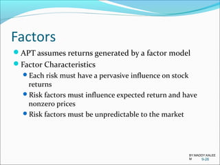
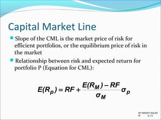
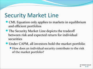
12. Capital Market Line
Line from RF to L is
capital market line
(CML)
x = risk premium
=E(RM) - RF
y =risk =σM
Slope =x/y
=[E(RM) - RF]/σM
y-intercept = RF
9-12
E(RM)
RF
Risk
σM
L
M
y
x
BY:MADDY.KALEE
M

13. The Separation Theorem
Investors use their preferences (reflected in an
indifference curve) to determine their optimal
portfolio
Separation Theorem:
The investment decision, which risky portfolio to
hold, is separate from the financing decision
Allocation between risk-free asset and risky
portfolio separate from choice of risky portfolio, T
9-13
BY:MADDY.KALEE
M

14. Separation Theorem
All investors
Invest in the same portfolio
Attain any point on the straight line RF-T-L by by either
borrowing or lending at the rate RF, depending on their
preferences
Risky portfolios are not tailored to each individual’s
taste
9-14
BY:MADDY.KALEE
M

15. Capital Market Line
Slope of the CML is the market price of risk for
efficient portfolios, or the equilibrium price of risk in
the market
Relationship between risk and expected return for
portfolio P (Equation for CML):
9-15
p
M
M
p σ
σ
RF)E(R
RF)E(R
−
+=
BY:MADDY.KALEE
M

16. Security Market Line
CML Equation only applies to markets in equilibrium
and efficient portfolios
The Security Market Line depicts the tradeoff
between risk and expected return for individual
securities
Under CAPM, all investors hold the market portfolio
How does an individual security contribute to the risk
of the market portfolio?
9-16
BY:MADDY.KALEE
M

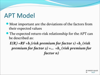
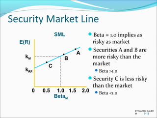
17. Security Market Line
A security’s contribution to the risk of the market
portfolio is based on beta
Equation for expected return for an individual stock
9-17
[ ]RF)E(RβRF)E(R Mii −+=
BY:MADDY.KALEE
M

18. Security Market Line
Beta = 1.0 implies as
risky as market
Securities A and B are
more risky than the
market
Beta >1.0
Security C is less risky
than the market
Beta <1.0
9-18
A
B
C
kM
kRF
0 1.0 2.00.5 1.5
SML
BetaM
E(R)
BY:MADDY.KALEE
M

19. Security Market Line
Beta measures systematic risk
Measures relative risk compared to the market portfolio
of all stocks
Volatility different than market
All securities should lie on the SML
The expected return on the security should be only that
return needed to compensate for systematic risk
9-19
BY:MADDY.KALEE
M

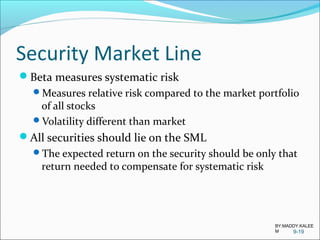
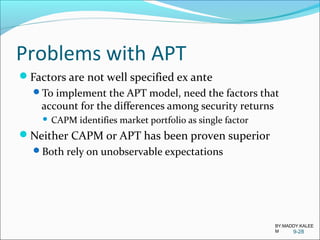
20. CAPM’s Expected
Return-Beta Relationship
Required rate of return on an asset (ki) is composed of
risk-free rate (RF)
risk premium (βi [ E(RM) - RF ])
 Market risk premium adjusted for specific security
ki = RF +βi [ E(RM) - RF ]
The greater the systematic risk, the greater the required
return
9-20
BY:MADDY.KALEE
M

21. Estimating the SML
Treasury Bill rate used to estimate RF
Expected market return unobservable
Estimated using past market returns and taking an
expected value
Estimating individual security betas difficult
Only company-specific factor in CAPM
Requires asset-specific forecast
9-21
BY:MADDY.KALEE
M

22. Estimating Beta
Market model
Relates the return on each stock to the return on the
market, assuming a linear relationship
Ri =αi +βi RM +ei
Characteristic line
Line fit to total returns for a security relative to total
returns for the market index
9-22
BY:MADDY.KALEE
M

23. How Accurate Are Beta Estimates?Betas change with a company’s situation
Not stationary over time
Estimating a future beta
May differ from the historical beta
RM represents the total of all marketable assets in the
economy
Approximated with a stock market index
Approximates return on all common stocks
9-23
BY:MADDY.KALEE
M

24. How Accurate Are Beta Estimates?
No one correct number of observations and time
periods for calculating beta
The regression calculations of the true α and β from
the characteristic line are subject to estimation error
Portfolio betas more reliable than individual security
betas
9-24
BY:MADDY.KALEE
M

25. Arbitrage Pricing Theory
Based on the Law of One Price
Two otherwise identical assets cannot sell at different
prices
Equilibrium prices adjust to eliminate all arbitrage
opportunities
Unlike CAPM, APT does not assume
single-period investment horizon, absence of personal
taxes, riskless borrowing or lending, mean-variance
decisions
9-25
BY:MADDY.KALEE
M

26. Factors
APT assumes returns generated by a factor model
Factor Characteristics
Each risk must have a pervasive influence on stock
returns
Risk factors must influence expected return and have
nonzero prices
Risk factors must be unpredictable to the market
9-26
BY:MADDY.KALEE
M

27. APT Model
Most important are the deviations of the factors from
their expected values
The expected return-risk relationship for the APT can
be described as:
E(Ri) =RF +bi1(risk premium for factor 1) +bi2 (risk
premium for factor 2) +… +bin (risk premium for
factor n)
9-27
BY:MADDY.KALEE
M

28. Problems with APT
Factors are not well specified ex ante
To implement the APT model, need the factors that
account for the differences among security returns
 CAPM identifies market portfolio as single factor
Neither CAPM or APT has been proven superior
Both rely on unobservable expectations
9-28
BY:MADDY.KALEE
M

29. Copyright 2006 John Wiley & Sons, Inc. All rights reserved.
Reproduction or translation of this work beyond that permitted in
Section 117 of the 1976 United states Copyright Act without the
express written permission of the copyright owner is unlawful.
Request for further information should be addressed to the
Permissions department, John Wiley & Sons, Inc. The purchaser
may make back-up copies for his/her own use only and not for
distribution or resale. The Publisher assumes no responsibility for
errors, omissions, or damages, caused by the use of these programs
or from the use of the information contained herein.
9-29
BY:MADDY.KALEE
M