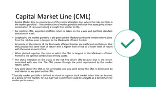
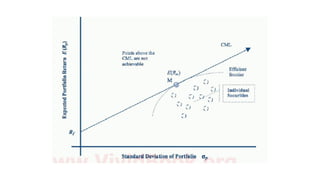
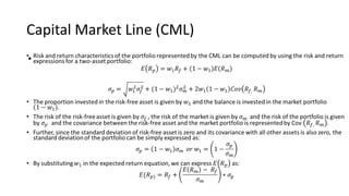
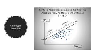
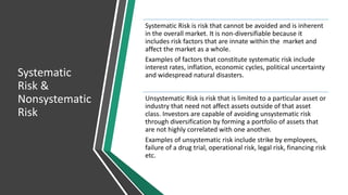
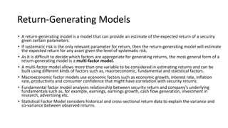
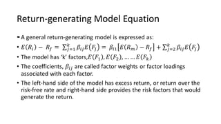
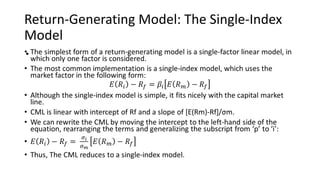
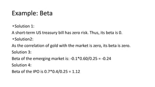
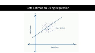
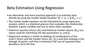
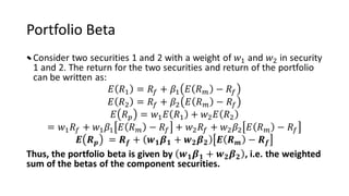
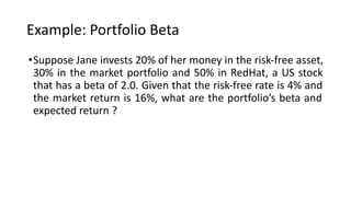
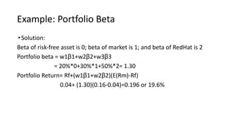
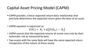
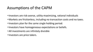
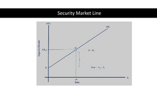
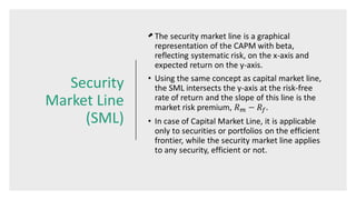
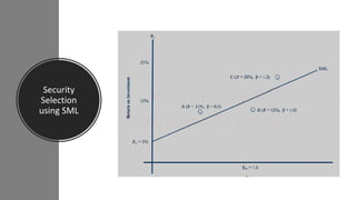
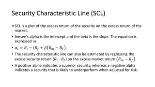
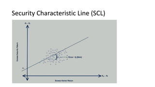
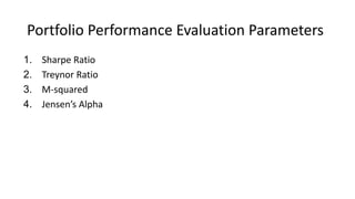
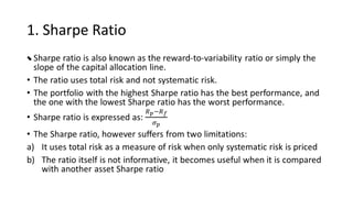
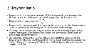
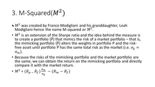
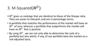
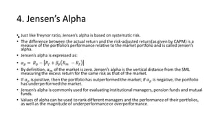
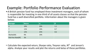
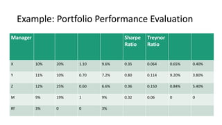
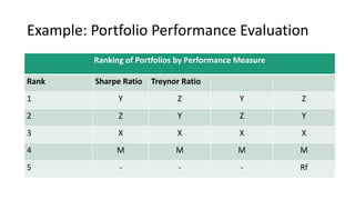
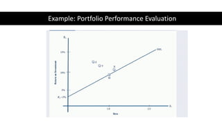
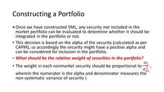
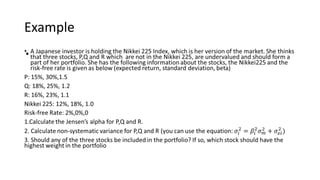
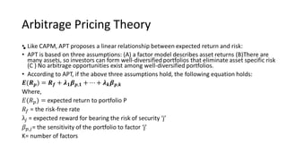
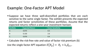
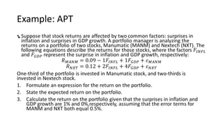
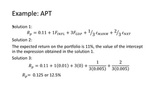
The document discusses various models for analyzing portfolio risk and return, including the Capital Market Line (CML) and different types of return-generating models. It also covers the Capital Asset Pricing Model (CAPM) and its assumptions, the Security Market Line (SML), and techniques for evaluating portfolio performance such as the Sharpe Ratio and Treynor Ratio. The Fama-French three-factor model and Carhart four-factor model, which extend the CAPM, are also summarized.

1. Portfolio Risk & Return: Part 2

2. Capital Market Line (CML)
• Capital Market Line is a special case of the capital allocation line, where the risky portfolio is
the market portfolio*. The combination of market portfolio with risk-free asset gives a linear
combination of two assets along a straight line, similar to CAL.
• For plotting CML, expected portfolio return is taken on the y-axis and portfolio standard
deviation on x-axis.
• Graphically, the market portfolio is the point on the Markowitz efficient frontier where a line
from the risk-free asset is tangent to the Markowitz efficient frontier.
• All points on the interior of the Markowitz efficient frontier are inefficient portfolios in that
they provide the same level of return with a higher level of risk or a lower level of return
with the same amount of risk.
• When plotted together, the point at which the CML is tangent to the Markowitz efficient
frontier is the optimal combination of risky assets.
• The CML’s intercept on the y-axis is the risk-free return (Rf) because that is the return
associated with zero risk. The CML passes through the point represented by the market
return, E(Rm).
• Any point above the CML is not achievable and any point below the CML is dominated by
and inferior to any point on the CML.
*Typically market portfolio is defined as a local or regional stock market index that can be used
as a proxy for the market, for e.g. S&P 500 is commonly used by analysts as a benchmark for
market performance.

4. Capital Market Line (CML)
•

5. Leveraged
Portfolios

6. Leveraged Portfolios
• The combination of the risk-free asset and the market portfolio, which may be
achieved by joining point RFR and M, are termed as ‘Lending Portfolios’. In
effect, the investor is lending part of his or her wealth at the risk-free rate.
• In case the investor wants to take more risk, he may be able to move to the
right of the market portfolio (point M) by borrowing money and purchasing
more of portfolio M.
• Assuming the investor is able to borrow at risk-free rate of interest, then the
straight line joining RFR and M can be extended further to the right of point
M, this extended section of the line represents the ‘Borrowing Portfolios’.
• As the investor moves further to the right of point M, an increasing amount of
borrowed money is invested in the market and this negative investment in the
risk-free asset is referred to as the ‘leveraged portfolios’.

7. Leveraged
Portfolios with
Different
Lending and
Borrowing
Rates

8. Leveraged
Portfolios with
Different
Lending &
Borrowing
Rates
•

9. Risk –
Meaning &
Pricing
Total
Variance
Unsystematic
Risk
Systematic Risk

10. Systematic
Risk &
Nonsystematic
Risk
Systematic Risk is risk that cannot be avoided and is inherent
in the overall market. It is non-diversifiable because it
includes risk factors that are innate within the market and
affect the market as a whole.
Examples of factors that constitute systematic risk include
interest rates, inflation, economic cycles, political uncertainty
and widespread natural disasters.
Unsystematic Risk is risk that is limited to a particular asset or
industry that need not affect assets outside of that asset
class. Investors are capable of avoiding unsystematic risk
through diversification by forming a portfolio of assets that
are not highly correlated with one another.
Examples of unsystematic risk include strike by employees,
failure of a drug trial, operational risk, legal risk, financing risk
etc.

11. Return-Generating Models
• A return-generating model is a model that can provide an estimate of the expected return of a security
given certain parameters.
• If systematic risk is the only relevant parameter for return, then the return-generating model will estimate
the expected return for any asset given the level of systematic risk.
• As it is difficult to decide which factors are appropriate for generating returns, the most general form of a
return-generating model is a multi-factor model.
• A multi-factor model allows more than one variable to be considered in estimating returns and can be
built using different kinds of factors such as, macroeconomic, fundamental and statistical factors.
• Macroeconomic factor models use economic factors such as economic growth, interest rate, inflation
rate, productivity and consumer confidence that might have correlation with security returns.
• Fundamental factor model analyses relationship between security return and company’s underlying
fundamentals such as, for example, earnings, earnings growth, cash flow generation, investment in
research, advertising etc.
• Statistical Factor Model considers historical and cross-sectional return data to explain the variance and
co-variance between observed returns.

12. Return-generating Model Equation
•

13. Return-Generating Model: The Single-Index
Model
•

14. Decomposition
of Total Risk for
a Single-Index
Model

15. Decomposition
of Total Risk for
a Single-Index
Model

16. Return-Generating Models: the Market
Model
•

17. Calculation & Interpretation of Beta
•

18. Example: Beta
•Assuming that the risk of the market is 25%, calculate the beta for the
following assets:
1. A short-term US Treasury Bill
2. Gold, which has a standard deviation equal to the standard
deviation of the market but a zero correlation with the market.
3. A new emerging market that is not currently included in the
definition of “market”- the emerging market’s standard deviation is
60% and the correlation with the market is -0.1.
4. An IPO with standard deviation of 40% and a correlation with the
market of 0.7.

19. Example: Beta
•Solution 1:
A short-term US treasury bill has zero risk. Thus, its beta is 0.
•Solution2:
As the correlation of gold with the market is zero, its beta is zero.
Solution 3:
Beta of the emerging market is: -0.1*0.60/0.25 = -0.24
Solution 4:
Beta of the IPO is 0.7*0.4/0.25 = 1.12

20. Beta Estimation Using Regression

21. Beta Estimation Using Regression
•

22. Portfolio Beta
•

23. Example: Portfolio Beta
•Suppose Jane invests 20% of her money in the risk-free asset,
30% in the market portfolio and 50% in RedHat, a US stock
that has a beta of 2.0. Given that the risk-free rate is 4% and
the market return is 16%, what are the portfolio’s beta and
expected return ?

24. Example: Portfolio Beta
•Solution:
Beta of risk-free asset is 0; beta of market is 1; and beta of RedHat is 2
Portfolio beta = w1β1+w2β2+w3β3
= 20%*0+30%*1+50%*2= 1.30
Portfolio Return= Rf+(w1β1+w2β2)(E(Rm)-Rf)
0.04+ (1.30)(0.16-0.04)=0.196 or 19.6%

25. Capital Asset Pricing Model (CAPM)
•

26. Assumptions of the CAPM
•Investors are risk-averse, utility-maximizing, rational individuals
•Markets are frictionless, including no transaction costs and no taxes.
•Investors plan for the same single holding period.
•Investors have homogeneous expectations or beliefs.
•All investments are infinitely divisible
•Investors are price takers.

27. Security Market Line

28. Security
Market Line
(SML)
•

29. Security
Selection
using SML

30. Security Selection Using SML
•Potential investors can plot a security’s expected return and beta
against the SML and use this relationship to decide whether the
security is overvalued or undervalued in the market.
•All securities that reflect the consensus market view are points
directly on the SML(i.e. correctly valued).
•If a point representing the estimated return of an asset is above the
SML (i.e. points A and C), the asset has a low level of risk relative to
the amount of expected return and would be a good choice for
investment. This security is termed as ‘undervalued’.
•If the point representing a particular asset is below the SML(point B),
the stock is considered as ‘overvalued’.

31. Security Characteristic Line (SCL)
•

32. Security Characteristic Line (SCL)

33. Portfolio Performance Evaluation Parameters
1. Sharpe Ratio
2. Treynor Ratio
3. M-squared
4. Jensen’s Alpha

34. 1. Sharpe Ratio
•

35. 2. Treynor Ratio
•

36. •

37. •

38. 4. Jensen’s Alpha
•

39. Example: Portfolio Performance Evaluation
•
Manager Return σ β
X 10% 20% 1.1
Y 11% 10% 0.7
Z 12% 25% 0.6
Market(M) 9% 19%
Risk-free Rate(Rf) 3%

40. Example: Portfolio Performance Evaluation
Manager Sharpe
Ratio
Treynor
Ratio
X 10% 20% 1.10 9.6% 0.35 0.064 0.65% 0.40%
Y 11% 10% 0.70 7.2% 0.80 0.114 9.20% 3.80%
Z 12% 25% 0.60 6.6% 0.36 0.150 0.84% 5.40%
M 9% 19% 1 9% 0.32 0.06 0 0
Rf 3% 0 0 3%

41. Example: Portfolio Performance Evaluation
Ranking of Portfolios by Performance Measure
Rank Sharpe Ratio Treynor Ratio
1 Y Z Y Z
2 Z Y Z Y
3 X X X X
4 M M M M
5 - - - Rf

42. Example: Portfolio Performance Evaluation

43. Constructing a Portfolio
•

44. Example
•

45. Limitations of CAPM
•True market portfolio is not observable
•Proxy for a market portfolio
•Estimation of beta risk
•Poor predictability of returns
•Homogeneity in investor expectations is not true

46. Arbitrage Pricing Theory
•

47. Example: One-Factor APT Model
•
Portfolio Expected Return Factor Sensitivity
A 0.075 0.5
B 0.150 2.0
C 0.070 0.4

48. Example: APT
•

49. Example: APT
•

50. Fama & French Three Factor Model
• Kenneth French and Eugene Fama presented a paper, the cross-section of Expected Stock Returns
(1992), were they investigated variables that could explain cross-section expected stock returns
better than the beta value in the CAPM.
• They found two anomalies that the CAPM could not explain, it was the book-to-market equity
ratio (BE/ME) and the size of company (market capitalization).
• They discovered that size has a negative relationship between average returns and firm size and
also that stocks with high BE/ME ratios have higher average returns. (Fama & French 1992).
• They also tested other variables like leverage and earnings/price ratio. But it was the size and
BE/ME factor that showed the most promising results and it was these two variables that they
used to create the three-factor model.
• The three-factor formula is an extended version of the CAPM, the first factor is the same as in the
CAPM which is the beta value for the asset. But in the three-factor model it also exists two others
beta coefficients, this means that the beta is divided in to three beta coefficients. (Fama & French
1992)

51. Fama & French Three Factor Model
•

52. Carhart(1997) Four factor model
• Mark M. Carhart wrote a paper in 1997 where he presented the model as a tool
for valuating mutual funds. The paper based it work of what Fama and French did
with the three-factor model in early 90´s.
• Carhart looked at the previous research and decided to include the momentum
factor in to the three-factor model and he performed the regression analysis on
mutual funds instead of stocks which Fama and French used in their paper.
• The Carhart model can be viewed as a multifactor extension of the CAPM that
explicitly incorporates drivers of differences in expected returns among asset
variables that are viewed as anomalies from a pure CAPM perspective.
• From the perspective of Carhart model, size, value and momentum represent
systematic risk factors; exposure to them is expected to be compensated in the
marketplace in the form of differences in mean return.

53. Carhart(1997)
Four factor
model