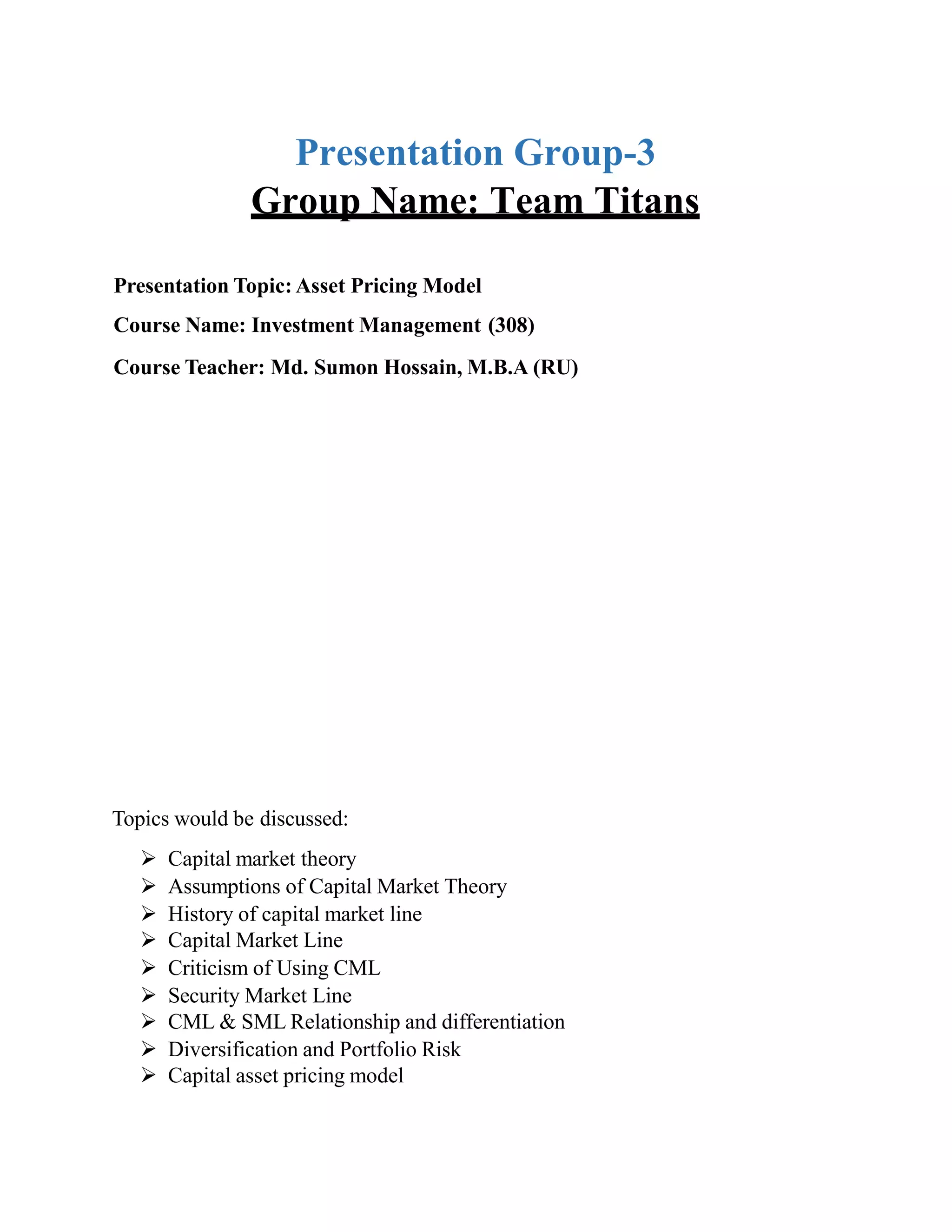
Presentation Group-3
Group Name: Team Titans
Presentation Topic: Asset Pricing Model
Course Name: Investment Management (308)
Course Teacher: Md. Sumon Hossain, M.B.A (RU)
Topics would be discussed:
 Capital market theory
 Assumptions of Capital Market Theory
 History of capital market line
 Capital Market Line
 Criticism of Using CML
 Security Market Line
 CML & SML Relationship and differentiation
 Diversification and Portfolio Risk
 Capital asset pricing model
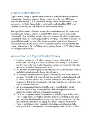
Capital Market theory
Capital market theory is a positive theory in that it hypothesis how investors do
behave rather than, how investors should behave, as, in the case of Modem
Portfolio Theory (MPT). It is reasonable "to view capital market" theory; as an
extension of portfolio theory, but it is important to understand that MPT is not
based on the validity, or lack thereof, of capital market theory.
The equilibrium model of interest to many investors is known as the capital asset
pricing model, typically referred to as the CAPM. It allows us to measure the
relevant risk of an individual security as well as to assess the relationship between
relevant risk of and the returns expected from investing. The CAPM is attractive as
an equilibrium model because of its simplicity and its implications. Because of
serious challenges, to the model, however, alternatives have been developed. The
primary alternative to the CAPM is arbitrage pricing theory, or APT, which allows
for multiple sources of risk.
Assumptions of Capital Market theory
 Investors can borrow or lend any amount of money at the risk-free rate of
return (RFR). (Clearly, it is always possible to lend money at the nominal
risk-free rate by buying risk free Securities such as government T-bills. It is
not always possible to borrow at this level.)
 All investors have homogeneous expectations; that is, they estimate identical
probability distributions for future rates of return.
 All investors have the same one-period time horizon, such as one month or
one year. The model will be developed for a single hypothetical period, and
its results could be affected by a different assumption since it requires
investors to derive risk measures and risk-free assets that are consistent with
their investment horizons.
 All investments are infinitely divisible, so it is possible to buy or sell
fractional shares of any asset or portfolio. This assumption allows us to
discuss investment alternatives as continuous curves.
 There are no taxes or transaction costs involved in buying or selling assets.
This is a reasonable assumption in many instances. Neither pension funds
nor charitable foundations have to pay taxes, and the transaction costs for
most financial institutions are negligible on most financial instruments.
 There is no inflation or any change in interest rates, or inflation is fully
anticipated. This is a reasonable initial assumption, and it can be modified.
 Capital markets are in equilibrium. This means that we begin with all
investments properly priced in line with their risk levels.
HISTORY OF CAPITAL MARKET LINE
Mean-variance analysis was pioneered by Harry Markowitz and james
Tobin. The efficient frontier of optimal portfolios was influenced by
Markowitz in 1952, and James Tobin included the risk free rate to mordern
portfolio theory in 1958. William Sharp then developed the CAPM in the
1960s, and won a nobel prize for his work in 1990, along with Markowitz
and Merton miller.
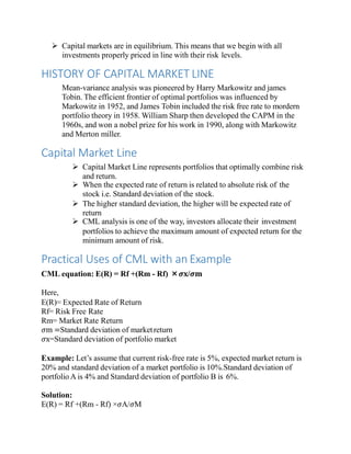
Capital Market Line
 Capital Market Line represents portfolios that optimally combine risk
and return.
 When the expected rate of return is related to absolute risk of the
stock i.e. Standard deviation of the stock.
 The higher standard deviation, the higher will be expected rate of
return
 CML analysis is one of the way, investors allocate their investment
portfolios to achieve the maximum amount of expected return for the
minimum amount of risk.
Practical Uses of CML with an Example
CML equation: E(R) = Rf +(Rm - Rf) ×𝝈𝐱/𝝈𝐦
Here,
E(R)= Expected Rate of Return
Rf= Risk Free Rate
Rm= Market Rate Return
𝜎m =Standard deviation of marketreturn
𝜎x=Standard deviation of portfolio market
Example: Let’s assume that current risk-free rate is 5%, expected market return is
20% and standard deviation of a market portfolio is 10%.Standard deviation of
portfolio A is 4% and Standard deviation of portfolio B is 6%.
Solution:
E(R) = Rf +(Rm - Rf) ×𝜎A/𝜎M
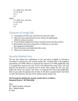
= 5+ (20%-5%) ×4%/10%
= 5+15×4/10
=5+6
=11
Again,
= 5+ (20%-5%) ×6%/10%
= 5+15×6/10
= 5+9
=14
Criticism of Using CML
 Assumption of CML may not hold true in the real world.
 There are taxes and transaction costs, which can significantly
differ for various investors.
 In real market conditions investors can lend at lower rate than borrow.
 Real markets don’t have strong form of efficiency, so investors
have unequal to information.
 Not all investors are rational and risks averse
 There are no risks free assets.
Security Market Line
The line that reflects the combination of risk and return available on alternative
investment is referred to as the security market line. Actually SML is the graphical
presentation of CAPM. When we represent the outcome of CAPM graphically, that
is, in graph there must be two axis. X axis will indicate beta values and y axis will
indicate risk premium or expected rate of return. Here, higher the risk you take,
higher the return you expect. And when we represent this total trend graphically,
then we get a plot of expected rate of return. It will show a upward trend. And when
we draw the trend line, this line will be called security market line.
The formula for plotting the security market line is as follows:
Required Return = Rf+(Rm-Rf)β
Here,
Rf = Risk Free Rate of Return
Rm = Market Return
β= Beta
Using the Security Market Line
The security market line is commonly used by investors in evaluating a security for
inclusion in an investment portfolio in terms of whether the security offers a
favorable expected return against its level of risk. When the security is plotted on
the SML chart, if it appears above the SML, it is considered undervalued because
the position on the chart indicates that the security offers a greater return against its
inherent risk. Conversely, if the security plots below the SML, it is considered
overvalued in price because the expected return does not overcome the inherentrisk.
The SML is frequently used in comparing two similar securities offering
approximately the same return, in order to determine which of the two securities
involves the least amount of inherent market risk in relation to the expected return.
The SML can also be used to compare securities of equal risk to see which one offers
the highest expected return against that level of risk.
CML & SML Similarities
 In both market lines, investments can be divided into unlimited pieces and
sizes.
 There are no taxes, inflation or transaction costs in both cases.
 Investors care only about returns created by their portfolios and individual
investments at the end of the period.
CML & SML Differentiation
Capital market line Securities Market Line
CML shows the rates of return and risk for a
specific portfolio
SML represents the market’s risk and return
and shows the expected returns of individual
assets.
Demonstrates market risk and return depending
on risk free rate of return and level of risks for
a specified portfolio.
Demonstrates the market risk and expected
rate of return at a given time.
The risk measure in the CML is the standard
deviation of returns (total risk).
While the measure of risk in the SML is
systematic risk, or beta.
Graphs drawn under Capital market line define
mostly, if not only, the efficient portfolios.
Security market line graph represents both
efficient and non-efficient portfolios.
Diversification and PortfolioRisk
 Market Risk
--Systematic or Non diversifiable.
 Firm-Specific Risk
--Non Systematic or Diversifiable.
How to Measure Diversification
A completely diversified portfolio would have a correlation with the market
portfolio of +1.00. This is logical because complete diversification means the
elimination of all the unsystematic or unique risk. Once this occurs, only systematic
risk is left, which cannot be diversified away. Therefore, completely diversified
portfolios would correlate perfectly with the market portfolio, which has only
systematic risk.
CAPITAL ASSET PRICING MODEL
The Capital Asset Pricing Model (CAPM) is a model that describes the
relationship between the expected return and risk of investing in a security. It
shows that the expected return on a security is equal to the risk-free return plus a
risk premium, which is based on the beta of that security.
CAPITAL ASSET PRICING MODEL ASSUMPTIONS
1. Investors are risk-averse, utility maximizing, rational individuals.
Risk aversion means investors expect to be compensated for bearing risk. Different
investors have different levels of risk aversion or risk tolerance.
Utility maximizing means investors prefer higher rate of returns to lower
returns.
Individuals are rational means that all investors have the ability to gather
and process information to make decisions.
2. Market are frictionless.
There are no transaction cost and no taxes.
Investors can borrow and lend as much as they want at risk-free rate.
One important assumption here is that there are no cost or restrictions on
short-selling, which is not true in reality.
3. All investors plan for the same, single holding period.
CAPM is based on a single period instead of multiple periods.
4. Investors have homogenous expectations.
All investors analyze securities using the same probability distribution to
arrive at identical valuations. This means all investors use the same estimates for
expected returns, variance and correlation between assets.
5. Investments are infinitely divisible.
Investors can hold a fraction of any asset. It means that they may invest
as much as or little in any asset.
6. Investors are price takers.
CAPM Formula and Calculation
CAPM is calculated according to the following formula:
Ri=Rf+(Rm-Rf) β
Here,
Ri=expected return of investment
Rf=Risk-free rate
Rm = Expected return of the market
β=Beta co efficient
(Rm-Rf)=Risk premium
Example: If the risk free rate is 5%, the market return is 10%, and the stock’s beta
is 2, what would be the expected rate of return?
Solution:
Ri=Rf+(Rm-Rf) β
=5%+(10℅-5%)2
=15℅
THE END

CAPM

  • 1.
    Presentation Group-3 Group Name:Team Titans Presentation Topic: Asset Pricing Model Course Name: Investment Management (308) Course Teacher: Md. Sumon Hossain, M.B.A (RU) Topics would be discussed:  Capital market theory  Assumptions of Capital Market Theory  History of capital market line  Capital Market Line  Criticism of Using CML  Security Market Line  CML & SML Relationship and differentiation  Diversification and Portfolio Risk  Capital asset pricing model
  • 2.
    Capital Market theory Capitalmarket theory is a positive theory in that it hypothesis how investors do behave rather than, how investors should behave, as, in the case of Modem Portfolio Theory (MPT). It is reasonable "to view capital market" theory; as an extension of portfolio theory, but it is important to understand that MPT is not based on the validity, or lack thereof, of capital market theory. The equilibrium model of interest to many investors is known as the capital asset pricing model, typically referred to as the CAPM. It allows us to measure the relevant risk of an individual security as well as to assess the relationship between relevant risk of and the returns expected from investing. The CAPM is attractive as an equilibrium model because of its simplicity and its implications. Because of serious challenges, to the model, however, alternatives have been developed. The primary alternative to the CAPM is arbitrage pricing theory, or APT, which allows for multiple sources of risk. Assumptions of Capital Market theory  Investors can borrow or lend any amount of money at the risk-free rate of return (RFR). (Clearly, it is always possible to lend money at the nominal risk-free rate by buying risk free Securities such as government T-bills. It is not always possible to borrow at this level.)  All investors have homogeneous expectations; that is, they estimate identical probability distributions for future rates of return.  All investors have the same one-period time horizon, such as one month or one year. The model will be developed for a single hypothetical period, and its results could be affected by a different assumption since it requires investors to derive risk measures and risk-free assets that are consistent with their investment horizons.  All investments are infinitely divisible, so it is possible to buy or sell fractional shares of any asset or portfolio. This assumption allows us to discuss investment alternatives as continuous curves.  There are no taxes or transaction costs involved in buying or selling assets. This is a reasonable assumption in many instances. Neither pension funds nor charitable foundations have to pay taxes, and the transaction costs for most financial institutions are negligible on most financial instruments.  There is no inflation or any change in interest rates, or inflation is fully anticipated. This is a reasonable initial assumption, and it can be modified.
  • 3.
     Capital marketsare in equilibrium. This means that we begin with all investments properly priced in line with their risk levels. HISTORY OF CAPITAL MARKET LINE Mean-variance analysis was pioneered by Harry Markowitz and james Tobin. The efficient frontier of optimal portfolios was influenced by Markowitz in 1952, and James Tobin included the risk free rate to mordern portfolio theory in 1958. William Sharp then developed the CAPM in the 1960s, and won a nobel prize for his work in 1990, along with Markowitz and Merton miller. Capital Market Line  Capital Market Line represents portfolios that optimally combine risk and return.  When the expected rate of return is related to absolute risk of the stock i.e. Standard deviation of the stock.  The higher standard deviation, the higher will be expected rate of return  CML analysis is one of the way, investors allocate their investment portfolios to achieve the maximum amount of expected return for the minimum amount of risk. Practical Uses of CML with an Example CML equation: E(R) = Rf +(Rm - Rf) ×𝝈𝐱/𝝈𝐦 Here, E(R)= Expected Rate of Return Rf= Risk Free Rate Rm= Market Rate Return 𝜎m =Standard deviation of marketreturn 𝜎x=Standard deviation of portfolio market Example: Let’s assume that current risk-free rate is 5%, expected market return is 20% and standard deviation of a market portfolio is 10%.Standard deviation of portfolio A is 4% and Standard deviation of portfolio B is 6%. Solution: E(R) = Rf +(Rm - Rf) ×𝜎A/𝜎M
  • 4.
    = 5+ (20%-5%)×4%/10% = 5+15×4/10 =5+6 =11 Again, = 5+ (20%-5%) ×6%/10% = 5+15×6/10 = 5+9 =14 Criticism of Using CML  Assumption of CML may not hold true in the real world.  There are taxes and transaction costs, which can significantly differ for various investors.  In real market conditions investors can lend at lower rate than borrow.  Real markets don’t have strong form of efficiency, so investors have unequal to information.  Not all investors are rational and risks averse  There are no risks free assets. Security Market Line The line that reflects the combination of risk and return available on alternative investment is referred to as the security market line. Actually SML is the graphical presentation of CAPM. When we represent the outcome of CAPM graphically, that is, in graph there must be two axis. X axis will indicate beta values and y axis will indicate risk premium or expected rate of return. Here, higher the risk you take, higher the return you expect. And when we represent this total trend graphically, then we get a plot of expected rate of return. It will show a upward trend. And when we draw the trend line, this line will be called security market line. The formula for plotting the security market line is as follows: Required Return = Rf+(Rm-Rf)β Here, Rf = Risk Free Rate of Return Rm = Market Return β= Beta
  • 5.
    Using the SecurityMarket Line The security market line is commonly used by investors in evaluating a security for inclusion in an investment portfolio in terms of whether the security offers a favorable expected return against its level of risk. When the security is plotted on the SML chart, if it appears above the SML, it is considered undervalued because the position on the chart indicates that the security offers a greater return against its inherent risk. Conversely, if the security plots below the SML, it is considered overvalued in price because the expected return does not overcome the inherentrisk. The SML is frequently used in comparing two similar securities offering approximately the same return, in order to determine which of the two securities involves the least amount of inherent market risk in relation to the expected return. The SML can also be used to compare securities of equal risk to see which one offers the highest expected return against that level of risk. CML & SML Similarities  In both market lines, investments can be divided into unlimited pieces and sizes.  There are no taxes, inflation or transaction costs in both cases.  Investors care only about returns created by their portfolios and individual investments at the end of the period. CML & SML Differentiation Capital market line Securities Market Line CML shows the rates of return and risk for a specific portfolio SML represents the market’s risk and return and shows the expected returns of individual assets. Demonstrates market risk and return depending on risk free rate of return and level of risks for a specified portfolio. Demonstrates the market risk and expected rate of return at a given time. The risk measure in the CML is the standard deviation of returns (total risk). While the measure of risk in the SML is systematic risk, or beta.
  • 6.
    Graphs drawn underCapital market line define mostly, if not only, the efficient portfolios. Security market line graph represents both efficient and non-efficient portfolios. Diversification and PortfolioRisk  Market Risk --Systematic or Non diversifiable.  Firm-Specific Risk --Non Systematic or Diversifiable. How to Measure Diversification A completely diversified portfolio would have a correlation with the market portfolio of +1.00. This is logical because complete diversification means the elimination of all the unsystematic or unique risk. Once this occurs, only systematic risk is left, which cannot be diversified away. Therefore, completely diversified portfolios would correlate perfectly with the market portfolio, which has only systematic risk. CAPITAL ASSET PRICING MODEL The Capital Asset Pricing Model (CAPM) is a model that describes the relationship between the expected return and risk of investing in a security. It shows that the expected return on a security is equal to the risk-free return plus a risk premium, which is based on the beta of that security. CAPITAL ASSET PRICING MODEL ASSUMPTIONS 1. Investors are risk-averse, utility maximizing, rational individuals. Risk aversion means investors expect to be compensated for bearing risk. Different investors have different levels of risk aversion or risk tolerance. Utility maximizing means investors prefer higher rate of returns to lower returns.
  • 7.
    Individuals are rationalmeans that all investors have the ability to gather and process information to make decisions. 2. Market are frictionless. There are no transaction cost and no taxes. Investors can borrow and lend as much as they want at risk-free rate. One important assumption here is that there are no cost or restrictions on short-selling, which is not true in reality. 3. All investors plan for the same, single holding period. CAPM is based on a single period instead of multiple periods. 4. Investors have homogenous expectations. All investors analyze securities using the same probability distribution to arrive at identical valuations. This means all investors use the same estimates for expected returns, variance and correlation between assets. 5. Investments are infinitely divisible. Investors can hold a fraction of any asset. It means that they may invest as much as or little in any asset. 6. Investors are price takers. CAPM Formula and Calculation CAPM is calculated according to the following formula: Ri=Rf+(Rm-Rf) β Here, Ri=expected return of investment Rf=Risk-free rate Rm = Expected return of the market β=Beta co efficient
  • 8.
    (Rm-Rf)=Risk premium Example: Ifthe risk free rate is 5%, the market return is 10%, and the stock’s beta is 2, what would be the expected rate of return? Solution: Ri=Rf+(Rm-Rf) β =5%+(10℅-5%)2 =15℅ THE END