Principles of Investing
FIN 330
CHAPTER 17
MODERN PORTFOLIO THEORY
CAPITAL ASSET PRICING THEORY
Dr David P Echevarria All Rights Reserved 1
STUDENT LEARNING OBJECTIVES
A. What is investment risk?
B. What is Modern Portfolio Theory (MPT)
C. What does MPT tell us about managing risk
and diversification?
D. What is the Capital Asset Pricing Model?
E. How does CAPM describe the efficient
frontier?
Dr David P Echevarria All Rights Reserved 2
INVESTMENT RISK
A. The probability of losing some or all of your
investment
B. Risk is a function of the dispersion of
possible future outcomes
1. Expected Value: probability of a particular
outcome times the magnitude (Eq. 17-1)
2. Risk is measured as the standard deviation of
expected outcomes (Eq. 17-2)
Dr David P Echevarria All Rights Reserved 3
MODERN PORTFOLIO THEORY (H.
MARKOWITZ)
A. The expected return of a portfolio is a
weighted average of the expected returns of
each of the securities in the portfolio
E(Rp) = S Xi Ri
B. The weights (Xi) are equal to the percentage
of the portfolio’s value which is invested in
each security and Ri is the [expected] return
for each asset i in the portfolio.
Dr David P Echevarria All Rights Reserved 4
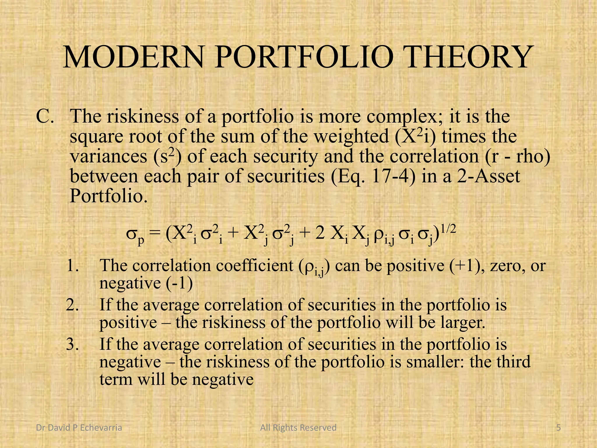
MODERN PORTFOLIO THEORY
C. The riskiness of a portfolio is more complex; it is the
square root of the sum of the weighted (X2i) times the
variances (s2) of each security and the correlation (r - rho)
between each pair of securities (Eq. 17-4) in a 2-Asset
Portfolio.
sp = (X2
i s2
i + X2
j s2
j + 2 Xi Xj ri,j si sj)1/2
1. The correlation coefficient (ri,j) can be positive (+1), zero, or
negative (-1)
2. If the average correlation of securities in the portfolio is
positive – the riskiness of the portfolio will be larger.
3. If the average correlation of securities in the portfolio is
negative – the riskiness of the portfolio is smaller: the third
term will be negative
Dr David P Echevarria All Rights Reserved 5
MODERN PORTFOLIO THEORY
D. MPT Efficient Portfolios
1. Efficient portfolios form a curvilinear frontier:
see Figure 17-3.
2. Assets that are efficiently price will fall on the
frontier as will all efficient portfolios.
3. In figure 17-3, assets D, E, and G are not
efficient – they lie below the E.F. These assets
are said to be overpriced. If the assets were
above the E.F., we would characterize them as
underpriced.
Dr David P Echevarria All Rights Reserved 6
MODERN PORTFOLIO THEORY
A. The following conclusions can be drawn:
1. When the holding period returns of two securities move in the
same direction, by the same amount at the same time, the pair
is perfectly positively correlated: rho = 1
2. When the holding period returns of two securities are totally
unrelated to each other, the pair is uncorrelated; rho = 0
3. The risk of a portfolio is the weighted average of the risk of
each security in the portfolio, and the correlations between
each pair of securities in the portfolio
4. Some textbooks use the covariance terms in the third term of
Eq. 17-4: si,j = ri,j si sj r = rho (r)
Dr David P Echevarria All Rights Reserved 7
Risk Reduction:
Benefits of Diversification
A. Portfolio diversification
1. Diversification can increase the risk/return tradeoff if the average
correlation coefficient between individual securities in the portfolio is
less than 1.0
2. The benefits of diversification increase as the correlation coefficient
gets smaller
B. Diversification across securities
1. As the number of securities in a portfolio increases the portfolio risk
decreases and approaches the risk of the total market
2. Market risk is inherent from business cycles, inflation, interest rates,
and economic factors
3. Firm-specific risk is tied to the company’s labor contracts, new
product development and other company related factors
Dr David P Echevarria All Rights Reserved 8
Risk Reduction:
Benefits of Diversification
C. Forms of Diversification
1. Mathematical: Increasing the number of stocks
reduces the portfolio risk
2. Diversification across time
3. Dollar cost averaging
4. Naive Diversification
a. Naive diversification occurs when investors select stocks at
random, and purchase and equal dollar amount of each
security
b. When N becomes large enough, naive diversification
averages out the firm-specific (unsystematic) risk of the
stocks in the portfolio, so that only the market (or
systematic) risk remains
Dr David P Echevarria All Rights Reserved 9
Capital Asset Pricing Model (CAPM)
A. Equation that defines the risk/return relationship
1. The CAPM assumes two assets: the risk-free asset and
the risky market portfolio
2. The two asset CAPM world results in a linear efficient
frontier: Capital Market Line (CML) See Figure 17-8
3. The risk aversion characteristic of the investor will
determine how much is invested in the risk-free asset and
how much is invested in the risky market portfolio
4. The standard deviation of the risk-free asset is zero.
5. Based on the idea that investors accept a higher risk only
for a higher return
Dr David P Echevarria All Rights Reserved 10
Capital Asset Pricing Model (CAPM)
B. Assumptions of the CAPM
1. Investors have cost-free and equal access to
information leading to homogenous expectations
2. Frictionless capital markets
a. No transaction costs or taxes (perfect)
b. Securities infinitely divisible (complete)
3. Investors are rational and seek to maximize their
expected utility functions
4. All investment is for the same time period
5. All investors can borrow or lend at the risk-free rate
Dr David P Echevarria All Rights Reserved 11
The Capital Market Line (CML)
A. Expected Portfolio Return:
E(Rp) = (X) E(Rp) + (1 - X) RF X = % Wealth Invested
B. Portfolio Risk: sP = S Xi sI
Where: Xi = proportion invested in asset i, si = the standard
deviation (riskiness) of asset i
1. Combinations of risk-free assets and risky portfolios can be used to
create portfolios along a line connecting the apex of the efficient
frontier and the risk-free rate
2. Describes the percentage holdings in the risk free asset and the risky
diversified market portfolio
3. The CML is also termed the Borrowing-Lending line, divided where
it intersects the efficient frontier (point M) with the lending line on
the lower left and borrowing on the upper right
A. v
Dr David P Echevarria All Rights Reserved 12
The Capital Market Line (CML)
C. The Market Portfolio
1. The Market Portfolio (point M) must be the only
risky portfolio chosen by all risk-averse
investors. Because it is demanded by all
investors, it must contain all the securities and
other traded assets
2. Portfolio M’s risk = Market risk
Dr David P Echevarria All Rights Reserved 13
The Capital Market Line (CML)
A. Measuring Relative Risk (Beta b)
1. Relative risk contribution of security i
2. Known as beta, b , it measures security risk, or
volatility relative to the market portfolio
a. Beta greater than 1.0 is riskier than the market
b. Beta less than 1.0 is less risky than the market
3. The value of beta implies something about
returns relative to the market portfolio
4. The choice of a proxy affects beta: e.g. S&P 500,
Wilshire 5000, Russell 1000, etc.
Dr David P Echevarria All Rights Reserved 14
The Capital Market Line (CML)
E. Types of CAPM Risk
1. Systematic or non-diversifiable risk: Beta is the measure of
systematic risk
2. Non-Systematic or diversifiable risk
a. Risk due to firm specific attributes
b. Become irrelevant in a well-diversified portfolio
c. Decisions made by total risk (standard deviations) instead of beta
ignore the systematic risk and diversifiable risk components of total
risk
F. The Security Market Line (SML)
1. The SML addresses the risk-return characteristics for
individual securities
2. The slope of the SML is equal to the stock’s beta coefficient.
Dr David P Echevarria All Rights Reserved 15
Fama and French Three-Factor
Model
A. The Fama and French model has three factors:
1. size of firms: Small minus Big (SMB)
2. book-to-market values: High minus Low (HML)
3. excess return on the market: Rp minus Rm (PMM)
B. The three factors:
1. SMB accounts for publicly traded companies with small
market caps that generate higher returns: Market Cap =
Price times Shares Outsg.
2. HML accounts for value stocks with high book-to-market
ratios that generate higher returns in comparison to the
market.
3. PMM account for the difference between the portfolio
return and the market return.
BARRA Risk Factor Analysis
(Barr Rosenberg, Barra Inc.)
A. Importance of Investment Risk
1. How investors and Pf managers measure investment risk
2. How to determine which assets worthy of investment.
B. Measures of Overall Risk (using 40 metrics)
1. Earnings Growth (~ PEG ratio)
2. Share Turnover
3. Senior Debt Rating (debentures)
4. Industry Risk
5. Company-specific Risk (idiosyncratic risk ~ variance/non-
market risk)
6. Other factors: Momentum, liquidity, leverage, size
Arbitrage Pricing Theory (APT)
A. APT is a multi-factor asset pricing model
1. that an asset's returns can be predicted using the linear
relationship between the asset’s expected return and a number
of macroeconomic variables that capture systematic risk. It is a
useful tool for analyzing portfolios from a value investing
perspective, in order to identify securities that may be
temporarily mispriced.
B. Arbitrage Pricing Theory Model: (simplified)
1. E(Ri)=E(Rz)+(E(i)−E(Rz))×βn
2. where:
a. E(R)i=Expected return on the asset i
b. Rz=Risk-Risk-Free rate of return
c. βn=Sensitivity of the asset price to macroeconomic factor n
d. Ei=Risk premium associated with factor i
Arbitrage Pricing Theory (APT)
C. Key Ideas
1. Arbitrage pricing theory (APT) is a multi-factor asset pricing
model
a. the idea that an asset's returns can be predicted using the linear
relationship between the asset’s expected return and a number (n) of
macroeconomic variables that capture systematic risk.
2. APT assumes markets sometimes misprice securities, before
the market eventually corrects and securities move back to fair
value.
a. CAPM assumes markets are perfectly efficient (mean and variance)
3. Because APT does not assume efficient markets, arbitrageurs
hope to take advantage of any deviations from fair market
value.
Arbitrage Pricing Theory (APT)
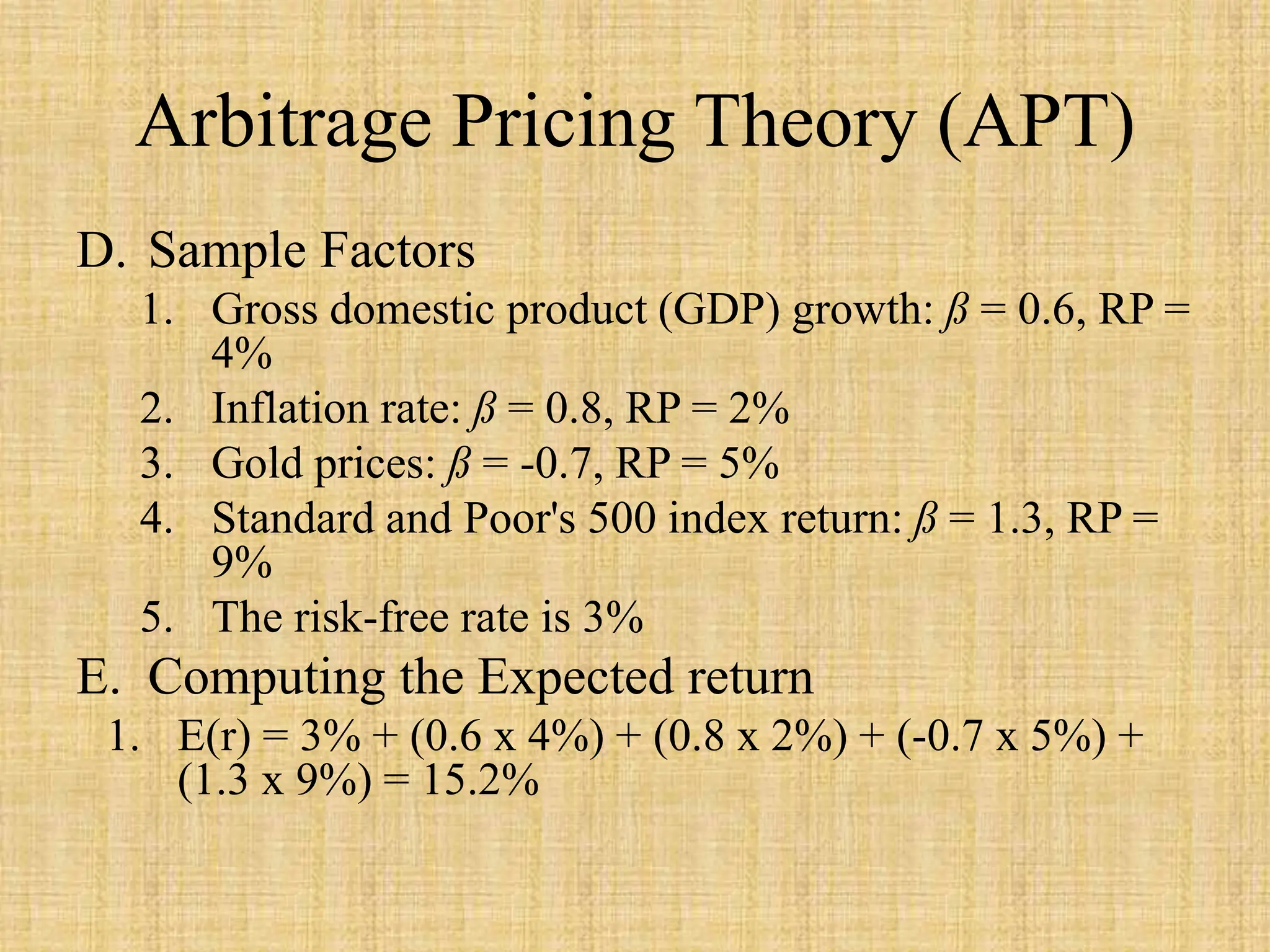
D. Sample Factors
1. Gross domestic product (GDP) growth: ß = 0.6, RP =
4%
2. Inflation rate: ß = 0.8, RP = 2%
3. Gold prices: ß = -0.7, RP = 5%
4. Standard and Poor's 500 index return: ß = 1.3, RP =
9%
5. The risk-free rate is 3%
E. Computing the Expected return
1. E(r) = 3% + (0.6 x 4%) + (0.8 x 2%) + (-0.7 x 5%) +
(1.3 x 9%) = 15.2%
HOMEWORK
A. Questions: 1, 5, 7, 9, 12
Dr David P Echevarria All Rights Reserved 21

Principal of investment and Portfolio Management

  • 1.
    Principles of Investing FIN330 CHAPTER 17 MODERN PORTFOLIO THEORY CAPITAL ASSET PRICING THEORY Dr David P Echevarria All Rights Reserved 1
  • 2.
    STUDENT LEARNING OBJECTIVES A.What is investment risk? B. What is Modern Portfolio Theory (MPT) C. What does MPT tell us about managing risk and diversification? D. What is the Capital Asset Pricing Model? E. How does CAPM describe the efficient frontier? Dr David P Echevarria All Rights Reserved 2
  • 3.
    INVESTMENT RISK A. Theprobability of losing some or all of your investment B. Risk is a function of the dispersion of possible future outcomes 1. Expected Value: probability of a particular outcome times the magnitude (Eq. 17-1) 2. Risk is measured as the standard deviation of expected outcomes (Eq. 17-2) Dr David P Echevarria All Rights Reserved 3
  • 4.
    MODERN PORTFOLIO THEORY(H. MARKOWITZ) A. The expected return of a portfolio is a weighted average of the expected returns of each of the securities in the portfolio E(Rp) = S Xi Ri B. The weights (Xi) are equal to the percentage of the portfolio’s value which is invested in each security and Ri is the [expected] return for each asset i in the portfolio. Dr David P Echevarria All Rights Reserved 4
  • 5.
    MODERN PORTFOLIO THEORY C.The riskiness of a portfolio is more complex; it is the square root of the sum of the weighted (X2i) times the variances (s2) of each security and the correlation (r - rho) between each pair of securities (Eq. 17-4) in a 2-Asset Portfolio. sp = (X2 i s2 i + X2 j s2 j + 2 Xi Xj ri,j si sj)1/2 1. The correlation coefficient (ri,j) can be positive (+1), zero, or negative (-1) 2. If the average correlation of securities in the portfolio is positive – the riskiness of the portfolio will be larger. 3. If the average correlation of securities in the portfolio is negative – the riskiness of the portfolio is smaller: the third term will be negative Dr David P Echevarria All Rights Reserved 5
  • 6.
    MODERN PORTFOLIO THEORY D.MPT Efficient Portfolios 1. Efficient portfolios form a curvilinear frontier: see Figure 17-3. 2. Assets that are efficiently price will fall on the frontier as will all efficient portfolios. 3. In figure 17-3, assets D, E, and G are not efficient – they lie below the E.F. These assets are said to be overpriced. If the assets were above the E.F., we would characterize them as underpriced. Dr David P Echevarria All Rights Reserved 6
  • 7.
    MODERN PORTFOLIO THEORY A.The following conclusions can be drawn: 1. When the holding period returns of two securities move in the same direction, by the same amount at the same time, the pair is perfectly positively correlated: rho = 1 2. When the holding period returns of two securities are totally unrelated to each other, the pair is uncorrelated; rho = 0 3. The risk of a portfolio is the weighted average of the risk of each security in the portfolio, and the correlations between each pair of securities in the portfolio 4. Some textbooks use the covariance terms in the third term of Eq. 17-4: si,j = ri,j si sj r = rho (r) Dr David P Echevarria All Rights Reserved 7
  • 8.
    Risk Reduction: Benefits ofDiversification A. Portfolio diversification 1. Diversification can increase the risk/return tradeoff if the average correlation coefficient between individual securities in the portfolio is less than 1.0 2. The benefits of diversification increase as the correlation coefficient gets smaller B. Diversification across securities 1. As the number of securities in a portfolio increases the portfolio risk decreases and approaches the risk of the total market 2. Market risk is inherent from business cycles, inflation, interest rates, and economic factors 3. Firm-specific risk is tied to the company’s labor contracts, new product development and other company related factors Dr David P Echevarria All Rights Reserved 8
  • 9.
    Risk Reduction: Benefits ofDiversification C. Forms of Diversification 1. Mathematical: Increasing the number of stocks reduces the portfolio risk 2. Diversification across time 3. Dollar cost averaging 4. Naive Diversification a. Naive diversification occurs when investors select stocks at random, and purchase and equal dollar amount of each security b. When N becomes large enough, naive diversification averages out the firm-specific (unsystematic) risk of the stocks in the portfolio, so that only the market (or systematic) risk remains Dr David P Echevarria All Rights Reserved 9
  • 10.
    Capital Asset PricingModel (CAPM) A. Equation that defines the risk/return relationship 1. The CAPM assumes two assets: the risk-free asset and the risky market portfolio 2. The two asset CAPM world results in a linear efficient frontier: Capital Market Line (CML) See Figure 17-8 3. The risk aversion characteristic of the investor will determine how much is invested in the risk-free asset and how much is invested in the risky market portfolio 4. The standard deviation of the risk-free asset is zero. 5. Based on the idea that investors accept a higher risk only for a higher return Dr David P Echevarria All Rights Reserved 10
  • 11.
    Capital Asset PricingModel (CAPM) B. Assumptions of the CAPM 1. Investors have cost-free and equal access to information leading to homogenous expectations 2. Frictionless capital markets a. No transaction costs or taxes (perfect) b. Securities infinitely divisible (complete) 3. Investors are rational and seek to maximize their expected utility functions 4. All investment is for the same time period 5. All investors can borrow or lend at the risk-free rate Dr David P Echevarria All Rights Reserved 11
  • 12.
    The Capital MarketLine (CML) A. Expected Portfolio Return: E(Rp) = (X) E(Rp) + (1 - X) RF X = % Wealth Invested B. Portfolio Risk: sP = S Xi sI Where: Xi = proportion invested in asset i, si = the standard deviation (riskiness) of asset i 1. Combinations of risk-free assets and risky portfolios can be used to create portfolios along a line connecting the apex of the efficient frontier and the risk-free rate 2. Describes the percentage holdings in the risk free asset and the risky diversified market portfolio 3. The CML is also termed the Borrowing-Lending line, divided where it intersects the efficient frontier (point M) with the lending line on the lower left and borrowing on the upper right A. v Dr David P Echevarria All Rights Reserved 12
  • 13.
    The Capital MarketLine (CML) C. The Market Portfolio 1. The Market Portfolio (point M) must be the only risky portfolio chosen by all risk-averse investors. Because it is demanded by all investors, it must contain all the securities and other traded assets 2. Portfolio M’s risk = Market risk Dr David P Echevarria All Rights Reserved 13
  • 14.
    The Capital MarketLine (CML) A. Measuring Relative Risk (Beta b) 1. Relative risk contribution of security i 2. Known as beta, b , it measures security risk, or volatility relative to the market portfolio a. Beta greater than 1.0 is riskier than the market b. Beta less than 1.0 is less risky than the market 3. The value of beta implies something about returns relative to the market portfolio 4. The choice of a proxy affects beta: e.g. S&P 500, Wilshire 5000, Russell 1000, etc. Dr David P Echevarria All Rights Reserved 14
  • 15.
    The Capital MarketLine (CML) E. Types of CAPM Risk 1. Systematic or non-diversifiable risk: Beta is the measure of systematic risk 2. Non-Systematic or diversifiable risk a. Risk due to firm specific attributes b. Become irrelevant in a well-diversified portfolio c. Decisions made by total risk (standard deviations) instead of beta ignore the systematic risk and diversifiable risk components of total risk F. The Security Market Line (SML) 1. The SML addresses the risk-return characteristics for individual securities 2. The slope of the SML is equal to the stock’s beta coefficient. Dr David P Echevarria All Rights Reserved 15
  • 16.
    Fama and FrenchThree-Factor Model A. The Fama and French model has three factors: 1. size of firms: Small minus Big (SMB) 2. book-to-market values: High minus Low (HML) 3. excess return on the market: Rp minus Rm (PMM) B. The three factors: 1. SMB accounts for publicly traded companies with small market caps that generate higher returns: Market Cap = Price times Shares Outsg. 2. HML accounts for value stocks with high book-to-market ratios that generate higher returns in comparison to the market. 3. PMM account for the difference between the portfolio return and the market return.
  • 17.
    BARRA Risk FactorAnalysis (Barr Rosenberg, Barra Inc.) A. Importance of Investment Risk 1. How investors and Pf managers measure investment risk 2. How to determine which assets worthy of investment. B. Measures of Overall Risk (using 40 metrics) 1. Earnings Growth (~ PEG ratio) 2. Share Turnover 3. Senior Debt Rating (debentures) 4. Industry Risk 5. Company-specific Risk (idiosyncratic risk ~ variance/non- market risk) 6. Other factors: Momentum, liquidity, leverage, size
  • 18.
    Arbitrage Pricing Theory(APT) A. APT is a multi-factor asset pricing model 1. that an asset's returns can be predicted using the linear relationship between the asset’s expected return and a number of macroeconomic variables that capture systematic risk. It is a useful tool for analyzing portfolios from a value investing perspective, in order to identify securities that may be temporarily mispriced. B. Arbitrage Pricing Theory Model: (simplified) 1. E(Ri)=E(Rz)+(E(i)−E(Rz))×βn 2. where: a. E(R)i=Expected return on the asset i b. Rz=Risk-Risk-Free rate of return c. βn=Sensitivity of the asset price to macroeconomic factor n d. Ei=Risk premium associated with factor i
  • 19.
    Arbitrage Pricing Theory(APT) C. Key Ideas 1. Arbitrage pricing theory (APT) is a multi-factor asset pricing model a. the idea that an asset's returns can be predicted using the linear relationship between the asset’s expected return and a number (n) of macroeconomic variables that capture systematic risk. 2. APT assumes markets sometimes misprice securities, before the market eventually corrects and securities move back to fair value. a. CAPM assumes markets are perfectly efficient (mean and variance) 3. Because APT does not assume efficient markets, arbitrageurs hope to take advantage of any deviations from fair market value.
  • 20.
    Arbitrage Pricing Theory(APT) D. Sample Factors 1. Gross domestic product (GDP) growth: ß = 0.6, RP = 4% 2. Inflation rate: ß = 0.8, RP = 2% 3. Gold prices: ß = -0.7, RP = 5% 4. Standard and Poor's 500 index return: ß = 1.3, RP = 9% 5. The risk-free rate is 3% E. Computing the Expected return 1. E(r) = 3% + (0.6 x 4%) + (0.8 x 2%) + (-0.7 x 5%) + (1.3 x 9%) = 15.2%
  • 21.
    HOMEWORK A. Questions: 1,5, 7, 9, 12 Dr David P Echevarria All Rights Reserved 21