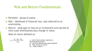
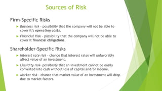
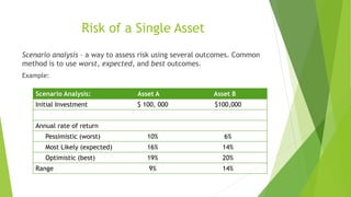
Principles of Managerial Finance
Quick overview of “Risk and Return” as part of
Principles of Managerial Finance course
Presentation Prepared
By Olga Shiryaeva
2015
Boston, MA
Risk and Return Fundamentals
 Portfolio – group of assets.
 Risk – likelihood of financial loss, also referred to as
uncertainty.
 Return – total gain or loss on an investment over period of
time (cash distributions plus change in value.
Rate of return defined as:
___________Ct + Pt – Pt-1
Pt-1
rt = rt – rate of return (actual, expected, or
required) during period t
Ct – cash flow received from asset investment
Pt – value of asset at t (time)
Pt-1 – value of asset t-1
Sources of Risk
Firm-Specific Risks
 Business risk – possibility that the company will not be able to
cover it’s operating costs.
 Financial Risk - possibility that the company will not be able to
cover it financial obligations.
Shareholder-Specific Risks
 Interest rate risk – chance that interest rates will unfavorably
affect value of an investment.
 Liquidity risk- possibility that an investment cannot be easily
converted into cash without loss of capital and/or income.
 Market risk – chance that market value of an investment will drop
due to market factors.
Sources of Risk (continued)
Firm and Shareholder Risks
 Event risk – possibility of an unforeseen event affecting the value
of the firm or a an investment.
 Exchange rate risk – chance of change in currency exchange rate,
unfavorably affecting the value of an investment.
 Purchasing power risk - chance that the cash flow from an
investment or firms value will be adversely affected due inflation
or deflation.
 Tax risk – possibility of changes in tax laws that could adversely
affect the value of the firm or an investment.
Risk Preference
 Risk-averse
Someone who avoids risk and requires more return for increased risk.
 Risk-indifferent
Someone who’s attitude (required or expected return) towards risk does
not change as risk increases.
 Risk-seeking
Someone who’s required return decreases as risk increases.
Risk preference – attitude of people towards risks.
Risk of a Single Asset
Scenario analysis – a way to assess risk using several outcomes. Common
method is to use worst, expected, and best outcomes.
Example:
Scenario Analysis: Asset A Asset B
Initial Investment $ 100, 000 $100,000
Annual rate of return
Pessimistic (worst) 10% 6%
Most Likely (expected) 16% 14%
Optimistic (best) 19% 20%
Range 9% 14%
Risk of a Single Asset (continued)
 Probability – chance that a given outcome will occur.
 Probability distribution – model that assigns probability to each possible
outcome.
 Continuous probability distribution – all the possible outcomes and their
associated probabilities.
Continuous Probability Distribution of three assets:
Risk of a Single Asset (continued)
 Standard deviation (σr) is used as a statistical indicator of assets risk.
It measures dispersion around expected value of return. Usually,
higher the standard deviation, the greater the risk.
 Expected value of return is the anticipated return on an asset.
 Normal probability distribution – probability distribution that is
symmetrical (”bell-shaped”).
 Coefficient of Variation(CV) used to determine volatility of an
investment. Higher CV indicates greater risk and therefore – higher
return.
Risk of a Single Asset (continued)
FORMULAS:
Expected value of return:
𝑟 = 𝑗=1
𝑛
𝑟𝑗* Prj , rj – return for the jth outcome
Prj – probability of occurrence of jth outcome
n – number of outcomes
Standard deviation of returns:
𝜎 𝑟 = 𝑗=1
𝑛
(𝑟𝑗 − 𝑟)2 * Prj
Coefficient of Variation:
CV =
σr
𝑟
Risk of a Single Asset (Example)
Expected Values of returnes for Assets 1 and 2
Possible
Outcomes
Probability (P) Returns (R) Weighted value
(PxR)
Asset 1
Pessimistic 0.15 11% 1.65%
Expected 0.55 13% 7.15%
Optimistic 0.30 15% 4.5%
Total 13.3%
Asset 2
Pessimistic 0.15 5% 0.75%
Expected 0.55 10% 5.5%
Optimistic 0.30 17% 5.1%
Total 11.35
Risk of a Single Asset (Example)
Standard Deviation for the returns of assets 1 and 2
j
(outcome)
rj
(return)
𝑟
(expectad value
of return)
rj - 𝑟 (rj - 𝑟)2 Prj
(probability of
occurrence)
(rj - 𝑟)2 x Prj
Asset 1
1 11% 13% -2% 4% 0.15 0.6%
2 13% 13% 0% 0% 0.55 0%
3 15% 13% 2% 4% 0.30 1.2%
Asset 2
1 5% 10% -5% 25% 0.15 3.75%
2 10% 10% 0% 0% 0.55 0%
3 17% 10% 7% 49% 0.30 14.7%
Risk of a Single Asset (Example)
Expected Return, Standard deviation, and Coefficient of variation
Statistics Asset 1 Asset 2
Expected Return (R) 13.3% 11.35%
Standard deviation (S) 8% 6%
Coefficient of variation (R/S) 1.6 1.9
Risk of a Portfolio
In reality any new investment is not evaluated independently
of other assets, but as a part of a portfolio.
Efficient Portfolio
Maximizes return
for a given level
of risk
or
Minimizes risk for
a given level of
return
Risk of a Portfolio (continued)
 Correlation - measures a relationship between two financial variables.
 Positively correlated – series move in the same direction (Example 1).
 Negatively correlated – series move in opposite directions (Example 2).
 Correlation coefficient – degree of correlation, ranges from +1 to -1.
A
B
Time
Example 1.
A
B
Example 2.
Risk of a Portfolio (continued)
 Diversification – combining assets that have negative or low
positive correlation to reduce overall risk of a portfolio.
 Uncorrelated assets - assets that have no interaction between
their returns.
 Correlation coefficient of uncorrelated assets is close to zero.
Asset A Asset B Portfolio of Assets A and B
Time Time Time
Return
Return
Return
Risk of a Portfolio (continued)
Example.
A company determined expected return and risk for assets A and B.
Possible Correlations.
Correlation Coefficient Ranges of return Ranges of Risk
Asset Expected Return Risk (standard deviation)
A 9% 4%
B 12% 7%
0 3 6 9 12
+1 (Perfect positive)
0 (Uncorrelated)
-1 (Perfect negative)
0 2 4 6 8
Portfolio return (%) Portfolio Risk (%)
The Capital Asset Pricing Model
(CAPM)
 The Capital Asset Pricing Model – describes the link between
risk and expected return.
 Total security risk = Nondiversifiable risk + Diversifiable risk
 Diversifiable risk (unsystematic) – company- or industry-specific
risk, such as a strike or a lawsuit that could negatively affect
price of company’s stock. It can be eliminated through
diversification.
 Nondiversifiable risk (systematic risk) – related to market
factors that affect whole industry. It cannot be eliminated
through diversification.
The Capital Asset Pricing Model
(CAPM) (continued)
CAPM links nondiversifiable risk and return.
Equation:
rj = RF + (bj x (rm - RF))
rj – required return on asset j
RF – rsik-free rate of return
bj – beta coefficient
rm – market return
The Capital Asset Pricing Model
(CAPM) (continued)
rj = RF + (bj x (rm - RF))
Risk-free rate
of return
Risk premium
Risk free rate of return – theoretically it is the minimum return
expected from any investment. In practice, interest rate of a three-
month U.S. Treasury bill is usually used as a risk free rate.
Risk premium – excess compensation that is expected in exchange for
extra risk.
The Capital Asset Pricing Model
(CAPM) (continued)
 Beta Coefficient – measures volatility of a security (or a portfolio). It
is an index that represents how return of an investment responds to a
change in the market return.
 Market return – combined return of all traded securities (for example
S&P 500).
Historical returns are used In order to calculate beta coefficient.
The Capital Asset Pricing Model
(CAPM) (continued)
Beta Derivation
Asset Return %
Market Return
0
- Data points representing historical market
returns (x) and asset returns (y).
The slope is beta
The Capital Asset Pricing Model
(CAPM) (continued)
 Market beta is considered to be 1.0
 Betas for assets can be positive or negative. Majority of betas are in the
range of 0.5 and 2.0
 Stock with a beta of 2.0 indicates that it is twice as responsive as a
market.
 Stock with a beta of 0.5 is half as responsive as market.
 Portfolio betas are interpreted just like beta for a single asset, but
considering the proportion of the total dollar value of every security.
 Generally, the higher the beta, the higher the required return, the lower
the beta, the lower the required return.
The Capital Asset Pricing Model
(CAPM) (continued)
Beta of a portfolio:
bp = 𝐣=𝟏
𝐧
𝐰𝐣 x 𝐛𝐣
wj – proportion of j-th asset (in $
value) as a part of the whole
portfolio
bj – beta of j-th asset
The Capital Asset Pricing Model
(CAPM) (continued)
 Graphically CAPM is represented as Security Market Line (SML).
 It represents amount of required return for each level of nondiversifiable
risk (beta).
0
Security Market Line
SML
Assets Risk
Premium 6%Market
Risk
Premium
3%
5
8
11
1 2
Nondiversifiable Risk, b
RequiredReturn,r(%)
The Capital Asset Pricing Model
(CAPM) (continued)
Position and slope of Security Market Line are affected by:
 Risk aversion
 Inflationary expectations
0
SML
5
8
11
1 2
RequiredReturn,r(%)
In graph to the left we can
see that 3% increase in
infationary expections
causes SML to shift upward,
which leads to 3% increase
in required return.
13
Change in inflationary expectations will result in corresponding change in the
returns of the assets.
The Capital Asset Pricing Model
(CAPM) (continued)
 The slope of Security Market Line represents the degree of risk aversion. The
steeper the slope of SML, the greater the risk premium in the market, which
also means the greater the degree of risk aversion.
 Risk premiums increase with increasing risk avoidance.
SML
5
8
11
13
Initial market risk
premium
New market risk
premium
Notes on CAPM.
Underlying assumptions and limitations.
 CAPM model relies on historic data. Betas are calculated using past
performance, therefore, they may or may not actually predict future returns.
 CAPM assumes efficient capital market, with many small investors (all rational
and risk-averse) have the same information and expectations, there are no
limitations on investments, with no taxes or transaction costs.
 It also assumes that all investors are fully diversified. However, in practice
that may not always be true.
 Although CAPM assumes all investors having the same time horizon, in
practice, however, all investors have different time horizons.
 Despite some of its drawbacks, CAPM is still an important framework used to
evaluate risk and return.
Sources Used:
Gitman L.J, “Principles of Managerial Finance”, 12th edition.
Investopedia, LLC. http://www.investopedia.com
McMenamin J., Financial Management: An Introduction.

Risk and return

  • 1.
    Principles of ManagerialFinance Quick overview of “Risk and Return” as part of Principles of Managerial Finance course Presentation Prepared By Olga Shiryaeva 2015 Boston, MA
  • 2.
    Risk and ReturnFundamentals  Portfolio – group of assets.  Risk – likelihood of financial loss, also referred to as uncertainty.  Return – total gain or loss on an investment over period of time (cash distributions plus change in value. Rate of return defined as: ___________Ct + Pt – Pt-1 Pt-1 rt = rt – rate of return (actual, expected, or required) during period t Ct – cash flow received from asset investment Pt – value of asset at t (time) Pt-1 – value of asset t-1
  • 3.
    Sources of Risk Firm-SpecificRisks  Business risk – possibility that the company will not be able to cover it’s operating costs.  Financial Risk - possibility that the company will not be able to cover it financial obligations. Shareholder-Specific Risks  Interest rate risk – chance that interest rates will unfavorably affect value of an investment.  Liquidity risk- possibility that an investment cannot be easily converted into cash without loss of capital and/or income.  Market risk – chance that market value of an investment will drop due to market factors.
  • 4.
    Sources of Risk(continued) Firm and Shareholder Risks  Event risk – possibility of an unforeseen event affecting the value of the firm or a an investment.  Exchange rate risk – chance of change in currency exchange rate, unfavorably affecting the value of an investment.  Purchasing power risk - chance that the cash flow from an investment or firms value will be adversely affected due inflation or deflation.  Tax risk – possibility of changes in tax laws that could adversely affect the value of the firm or an investment.
  • 5.
    Risk Preference  Risk-averse Someonewho avoids risk and requires more return for increased risk.  Risk-indifferent Someone who’s attitude (required or expected return) towards risk does not change as risk increases.  Risk-seeking Someone who’s required return decreases as risk increases. Risk preference – attitude of people towards risks.
  • 6.
    Risk of aSingle Asset Scenario analysis – a way to assess risk using several outcomes. Common method is to use worst, expected, and best outcomes. Example: Scenario Analysis: Asset A Asset B Initial Investment $ 100, 000 $100,000 Annual rate of return Pessimistic (worst) 10% 6% Most Likely (expected) 16% 14% Optimistic (best) 19% 20% Range 9% 14%
  • 7.
    Risk of aSingle Asset (continued)  Probability – chance that a given outcome will occur.  Probability distribution – model that assigns probability to each possible outcome.  Continuous probability distribution – all the possible outcomes and their associated probabilities. Continuous Probability Distribution of three assets:
  • 8.
    Risk of aSingle Asset (continued)  Standard deviation (σr) is used as a statistical indicator of assets risk. It measures dispersion around expected value of return. Usually, higher the standard deviation, the greater the risk.  Expected value of return is the anticipated return on an asset.  Normal probability distribution – probability distribution that is symmetrical (”bell-shaped”).  Coefficient of Variation(CV) used to determine volatility of an investment. Higher CV indicates greater risk and therefore – higher return.
  • 9.
    Risk of aSingle Asset (continued) FORMULAS: Expected value of return: 𝑟 = 𝑗=1 𝑛 𝑟𝑗* Prj , rj – return for the jth outcome Prj – probability of occurrence of jth outcome n – number of outcomes Standard deviation of returns: 𝜎 𝑟 = 𝑗=1 𝑛 (𝑟𝑗 − 𝑟)2 * Prj Coefficient of Variation: CV = σr 𝑟
  • 10.
    Risk of aSingle Asset (Example) Expected Values of returnes for Assets 1 and 2 Possible Outcomes Probability (P) Returns (R) Weighted value (PxR) Asset 1 Pessimistic 0.15 11% 1.65% Expected 0.55 13% 7.15% Optimistic 0.30 15% 4.5% Total 13.3% Asset 2 Pessimistic 0.15 5% 0.75% Expected 0.55 10% 5.5% Optimistic 0.30 17% 5.1% Total 11.35
  • 11.
    Risk of aSingle Asset (Example) Standard Deviation for the returns of assets 1 and 2 j (outcome) rj (return) 𝑟 (expectad value of return) rj - 𝑟 (rj - 𝑟)2 Prj (probability of occurrence) (rj - 𝑟)2 x Prj Asset 1 1 11% 13% -2% 4% 0.15 0.6% 2 13% 13% 0% 0% 0.55 0% 3 15% 13% 2% 4% 0.30 1.2% Asset 2 1 5% 10% -5% 25% 0.15 3.75% 2 10% 10% 0% 0% 0.55 0% 3 17% 10% 7% 49% 0.30 14.7%
  • 12.
    Risk of aSingle Asset (Example) Expected Return, Standard deviation, and Coefficient of variation Statistics Asset 1 Asset 2 Expected Return (R) 13.3% 11.35% Standard deviation (S) 8% 6% Coefficient of variation (R/S) 1.6 1.9
  • 13.
    Risk of aPortfolio In reality any new investment is not evaluated independently of other assets, but as a part of a portfolio. Efficient Portfolio Maximizes return for a given level of risk or Minimizes risk for a given level of return
  • 14.
    Risk of aPortfolio (continued)  Correlation - measures a relationship between two financial variables.  Positively correlated – series move in the same direction (Example 1).  Negatively correlated – series move in opposite directions (Example 2).  Correlation coefficient – degree of correlation, ranges from +1 to -1. A B Time Example 1. A B Example 2.
  • 15.
    Risk of aPortfolio (continued)  Diversification – combining assets that have negative or low positive correlation to reduce overall risk of a portfolio.  Uncorrelated assets - assets that have no interaction between their returns.  Correlation coefficient of uncorrelated assets is close to zero. Asset A Asset B Portfolio of Assets A and B Time Time Time Return Return Return
  • 16.
    Risk of aPortfolio (continued) Example. A company determined expected return and risk for assets A and B. Possible Correlations. Correlation Coefficient Ranges of return Ranges of Risk Asset Expected Return Risk (standard deviation) A 9% 4% B 12% 7% 0 3 6 9 12 +1 (Perfect positive) 0 (Uncorrelated) -1 (Perfect negative) 0 2 4 6 8 Portfolio return (%) Portfolio Risk (%)
  • 17.
    The Capital AssetPricing Model (CAPM)  The Capital Asset Pricing Model – describes the link between risk and expected return.  Total security risk = Nondiversifiable risk + Diversifiable risk  Diversifiable risk (unsystematic) – company- or industry-specific risk, such as a strike or a lawsuit that could negatively affect price of company’s stock. It can be eliminated through diversification.  Nondiversifiable risk (systematic risk) – related to market factors that affect whole industry. It cannot be eliminated through diversification.
  • 18.
    The Capital AssetPricing Model (CAPM) (continued) CAPM links nondiversifiable risk and return. Equation: rj = RF + (bj x (rm - RF)) rj – required return on asset j RF – rsik-free rate of return bj – beta coefficient rm – market return
  • 19.
    The Capital AssetPricing Model (CAPM) (continued) rj = RF + (bj x (rm - RF)) Risk-free rate of return Risk premium Risk free rate of return – theoretically it is the minimum return expected from any investment. In practice, interest rate of a three- month U.S. Treasury bill is usually used as a risk free rate. Risk premium – excess compensation that is expected in exchange for extra risk.
  • 20.
    The Capital AssetPricing Model (CAPM) (continued)  Beta Coefficient – measures volatility of a security (or a portfolio). It is an index that represents how return of an investment responds to a change in the market return.  Market return – combined return of all traded securities (for example S&P 500). Historical returns are used In order to calculate beta coefficient.
  • 21.
    The Capital AssetPricing Model (CAPM) (continued) Beta Derivation Asset Return % Market Return 0 - Data points representing historical market returns (x) and asset returns (y). The slope is beta
  • 22.
    The Capital AssetPricing Model (CAPM) (continued)  Market beta is considered to be 1.0  Betas for assets can be positive or negative. Majority of betas are in the range of 0.5 and 2.0  Stock with a beta of 2.0 indicates that it is twice as responsive as a market.  Stock with a beta of 0.5 is half as responsive as market.  Portfolio betas are interpreted just like beta for a single asset, but considering the proportion of the total dollar value of every security.  Generally, the higher the beta, the higher the required return, the lower the beta, the lower the required return.
  • 23.
    The Capital AssetPricing Model (CAPM) (continued) Beta of a portfolio: bp = 𝐣=𝟏 𝐧 𝐰𝐣 x 𝐛𝐣 wj – proportion of j-th asset (in $ value) as a part of the whole portfolio bj – beta of j-th asset
  • 24.
    The Capital AssetPricing Model (CAPM) (continued)  Graphically CAPM is represented as Security Market Line (SML).  It represents amount of required return for each level of nondiversifiable risk (beta). 0 Security Market Line SML Assets Risk Premium 6%Market Risk Premium 3% 5 8 11 1 2 Nondiversifiable Risk, b RequiredReturn,r(%)
  • 25.
    The Capital AssetPricing Model (CAPM) (continued) Position and slope of Security Market Line are affected by:  Risk aversion  Inflationary expectations 0 SML 5 8 11 1 2 RequiredReturn,r(%) In graph to the left we can see that 3% increase in infationary expections causes SML to shift upward, which leads to 3% increase in required return. 13 Change in inflationary expectations will result in corresponding change in the returns of the assets.
  • 26.
    The Capital AssetPricing Model (CAPM) (continued)  The slope of Security Market Line represents the degree of risk aversion. The steeper the slope of SML, the greater the risk premium in the market, which also means the greater the degree of risk aversion.  Risk premiums increase with increasing risk avoidance. SML 5 8 11 13 Initial market risk premium New market risk premium
  • 27.
    Notes on CAPM. Underlyingassumptions and limitations.  CAPM model relies on historic data. Betas are calculated using past performance, therefore, they may or may not actually predict future returns.  CAPM assumes efficient capital market, with many small investors (all rational and risk-averse) have the same information and expectations, there are no limitations on investments, with no taxes or transaction costs.  It also assumes that all investors are fully diversified. However, in practice that may not always be true.  Although CAPM assumes all investors having the same time horizon, in practice, however, all investors have different time horizons.  Despite some of its drawbacks, CAPM is still an important framework used to evaluate risk and return.
  • 28.
    Sources Used: Gitman L.J,“Principles of Managerial Finance”, 12th edition. Investopedia, LLC. http://www.investopedia.com McMenamin J., Financial Management: An Introduction.