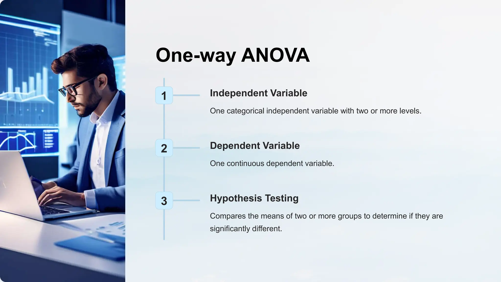
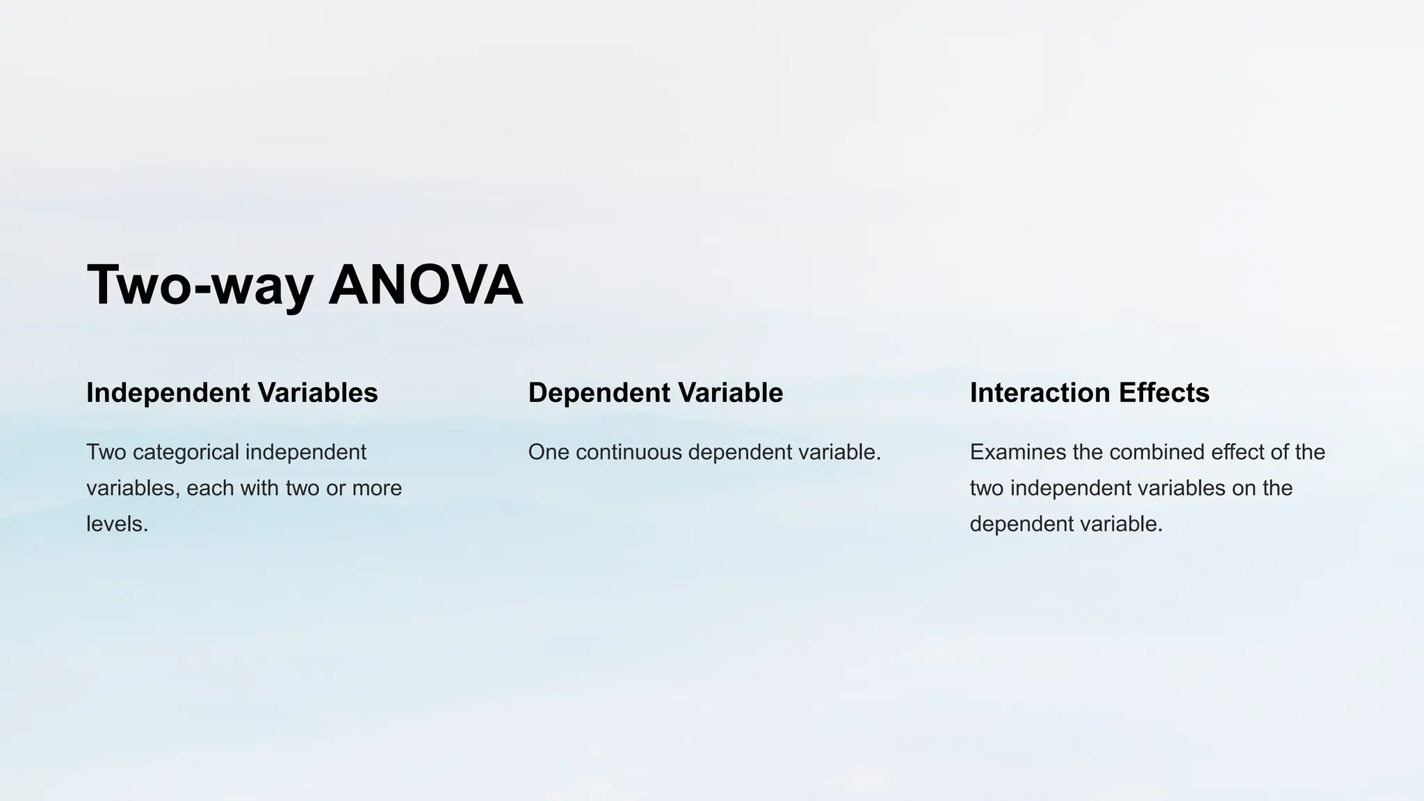
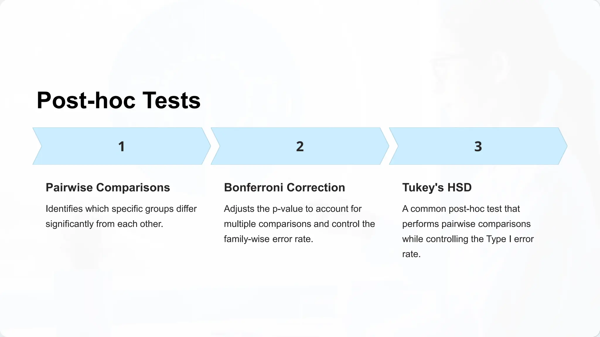
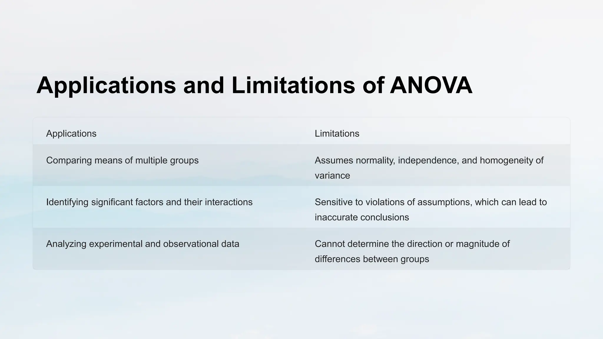
Introduction to
ANOVA
ANOVA, or Analysis of Variance, is a statistical technique used to
compare the means of two or more groups. It helps determine if there are
significant differences between the groups and identifies the sources of
variation.
By: Bunga Satya Hardika
Esti Sapta Lestari
Fajriati
Selza
Wahyu
Assumptions of ANOVA
1 Normality
The data in each group should
follow a normal distribution.
2 Independence
The observations in each group
should be independent of each
other.
3 Homogeneity of
Variance
The variances of the groups
should be equal.
Random Sampling
4
The data should be collected through a process of random
sampling to ensure that the sample represents the
population from which it was drawn.
5 Additivity
The model assumes that the effect of the different factors
is additive. This means that the combined effect of
different factors is equal to the sum of their individual
effects.
Here is a simple example of how ANOVA is used and
how the assumptions are checked:
Suppose we want to find out if there is a difference in average
test scores between three different classes. We have test score
data from 30 students divided into three classes (A, B, and C)
with 10 students each per class.
Step 1: Collecting Data
Suppose the exam score data is as follows:
Class A: 75, 80, 85, 70, 90, 95, 85, 80, 75, 85
Class B: 65, 70, 75, 60, 85, 70, 80, 75, 65, 70
Class C: 85, 90, 95, 80, 75, 85, 90, 85, 80, 75
Step 2: Checking Assumptions
1. Independence of Observations: The scores of each student in
different classes are assumed to be independent. For example,
the score of a student in Class A is not influenced by the score of
a student in Class B or C.
2. Normality: We check normality using the Shapiro-Wilk test or
by looking at the Q-Q plot.
3. Homogeneity of Variance: We check homogeneity of variance
using Levene's or Bartlett's test.
4. Random Sampling: Data is considered to be randomly drawn
from the population of students taking the exam.
5. Additivity: It is assumed that the effect of class on test scores
is additive.
Step 3: Performing ANOVA
We will use statistical software (such as Python, R, or SPSS) to
perform the ANOVA.
Step 4: Interpretation of Results
- If the p-value of the Shapiro-Wilk test for each class is greater
than 0.05, the normality assumption is met.
- If the p-value of the Levene's test is greater than 0.05, the
assumption of homogeneity of variance is met.
- The ANOVA results will show whether there is a significant
difference between the mean exam scores in the three classes.
If the p-value of the ANOVA result is smaller than 0.05, we
conclude that there is a significant difference between the
mean test scores in at least two classes.
Thus, these steps will help us understand how to use ANOVA and
ensure that the necessary assumptions are met.
One-way ANOVA
1 Independent Variable
One categorical independent variable with two or more levels.
2 Dependent Variable
One continuous dependent variable.
3 Hypothesis Testing
Compares the means of two or more groups to determine if they are
significantly different.
Two-way ANOVA
Independent Variables
Two categorical independent
variables, each with two or more
levels.
Dependent Variable
One continuous dependent variable.
Interaction Effects
Examines the combined effect of the
two independent variables on the
dependent variable.
Interpreting ANOVA Results
F-statistic
Compares the variance between groups to the variance
within groups.
p-value
Determines the statistical significance of the differences
between groups.
Effect Size
Quantifies the magnitude of the difference between
groups.
Interaction Effects
Indicates if the effect of one independent variable
depends on the level of the other independent variable.
Post-hoc Tests
Pairwise Comparisons
Identifies which specific groups differ
significantly from each other.
Bonferroni Correction
Adjusts the p-value to account for
multiple comparisons and control the
family-wise error rate.
Tukey's HSD
A common post-hoc test that
performs pairwise comparisons
while controlling the Type I error
rate.
Effect Size and Statistical Power
Effect Size
Quantifies the magnitude of the
difference between groups,
independent of sample size.
Statistical Power
The probability of detecting an effect if
it truly exists. Helps determine the
appropriate sample size.
Interpreting Results
Considering both statistical
significance and effect size provides a
more complete understanding of the
findings.
Applications and Limitations of ANOVA
Applications Limitations
Comparing means of multiple groups Assumes normality, independence, and homogeneity of
variance
Identifying significant factors and their interactions Sensitive to violations of assumptions, which can lead to
inaccurate conclusions
Analyzing experimental and observational data Cannot determine the direction or magnitude of
differences between groups

ppt anova analysis of varian presentation

  • 1.
    Introduction to ANOVA ANOVA, orAnalysis of Variance, is a statistical technique used to compare the means of two or more groups. It helps determine if there are significant differences between the groups and identifies the sources of variation. By: Bunga Satya Hardika Esti Sapta Lestari Fajriati Selza Wahyu
  • 2.
    Assumptions of ANOVA 1Normality The data in each group should follow a normal distribution. 2 Independence The observations in each group should be independent of each other. 3 Homogeneity of Variance The variances of the groups should be equal. Random Sampling 4 The data should be collected through a process of random sampling to ensure that the sample represents the population from which it was drawn. 5 Additivity The model assumes that the effect of the different factors is additive. This means that the combined effect of different factors is equal to the sum of their individual effects.
  • 3.
    Here is asimple example of how ANOVA is used and how the assumptions are checked: Suppose we want to find out if there is a difference in average test scores between three different classes. We have test score data from 30 students divided into three classes (A, B, and C) with 10 students each per class. Step 1: Collecting Data Suppose the exam score data is as follows: Class A: 75, 80, 85, 70, 90, 95, 85, 80, 75, 85 Class B: 65, 70, 75, 60, 85, 70, 80, 75, 65, 70 Class C: 85, 90, 95, 80, 75, 85, 90, 85, 80, 75 Step 2: Checking Assumptions 1. Independence of Observations: The scores of each student in different classes are assumed to be independent. For example, the score of a student in Class A is not influenced by the score of a student in Class B or C. 2. Normality: We check normality using the Shapiro-Wilk test or by looking at the Q-Q plot. 3. Homogeneity of Variance: We check homogeneity of variance using Levene's or Bartlett's test. 4. Random Sampling: Data is considered to be randomly drawn from the population of students taking the exam. 5. Additivity: It is assumed that the effect of class on test scores is additive. Step 3: Performing ANOVA We will use statistical software (such as Python, R, or SPSS) to perform the ANOVA. Step 4: Interpretation of Results - If the p-value of the Shapiro-Wilk test for each class is greater than 0.05, the normality assumption is met. - If the p-value of the Levene's test is greater than 0.05, the assumption of homogeneity of variance is met. - The ANOVA results will show whether there is a significant difference between the mean exam scores in the three classes. If the p-value of the ANOVA result is smaller than 0.05, we conclude that there is a significant difference between the mean test scores in at least two classes. Thus, these steps will help us understand how to use ANOVA and ensure that the necessary assumptions are met.
  • 4.
    One-way ANOVA 1 IndependentVariable One categorical independent variable with two or more levels. 2 Dependent Variable One continuous dependent variable. 3 Hypothesis Testing Compares the means of two or more groups to determine if they are significantly different.
  • 5.
    Two-way ANOVA Independent Variables Twocategorical independent variables, each with two or more levels. Dependent Variable One continuous dependent variable. Interaction Effects Examines the combined effect of the two independent variables on the dependent variable.
  • 6.
    Interpreting ANOVA Results F-statistic Comparesthe variance between groups to the variance within groups. p-value Determines the statistical significance of the differences between groups. Effect Size Quantifies the magnitude of the difference between groups. Interaction Effects Indicates if the effect of one independent variable depends on the level of the other independent variable.
  • 7.
    Post-hoc Tests Pairwise Comparisons Identifieswhich specific groups differ significantly from each other. Bonferroni Correction Adjusts the p-value to account for multiple comparisons and control the family-wise error rate. Tukey's HSD A common post-hoc test that performs pairwise comparisons while controlling the Type I error rate.
  • 8.
    Effect Size andStatistical Power Effect Size Quantifies the magnitude of the difference between groups, independent of sample size. Statistical Power The probability of detecting an effect if it truly exists. Helps determine the appropriate sample size. Interpreting Results Considering both statistical significance and effect size provides a more complete understanding of the findings.
  • 9.
    Applications and Limitationsof ANOVA Applications Limitations Comparing means of multiple groups Assumes normality, independence, and homogeneity of variance Identifying significant factors and their interactions Sensitive to violations of assumptions, which can lead to inaccurate conclusions Analyzing experimental and observational data Cannot determine the direction or magnitude of differences between groups