One Way ANOVA
Dr.Shovan padhy, MBBS, MD
DM 1st yr (Senior Resident)
NIMS, Hyderabad
Overview
• Introduction.
• Why ANOVA instead of multiple t-tests?
• One way ANOVA.
• Assumptions of One way ANOVA.
• Steps in One way ANOVA.
• Example.
• Conclusion.
Introduction
• ANOVA is an abbreviation for the full name of the method:
Analysis Of Variance.
• Invented by R.A. Fisher in the 1918.
• ANOVA is used to test the significance of the difference
between more than two sample means.
• Name “ANOVA” is a misnomer as it compares mean to check
variance between group.
Summary Table of Statistical tests
Level of
Measurement
Sample Characteristics
Correlation
1 Sample
2 Sample K Sample (i.e., >2)
Independent Dependent Independent Dependent
Categorical or
Nominal
Χ2 or
bi-
nomina
l
Χ2 Macnarmar’s
Χ2
Χ2 Cochran’s Q
Rank or
Ordinal
Mann
Whitney U
Wilcoxin
Matched
Pairs Signed
Ranks
Kruskal
Wallis H
Friedman’s
ANOVA
Spearman’s
rho
Parametric
(Interval &
Ratio)
z test
or
t test
t test
between
groups
t test
within
groups
1 way ANOVA
between
groups
1 way ANOVA
(within or
repeated
measure)
Pearson’s
r
Factorial (2 way) ANOVA
Χ2
Why ANOVA instead of multiple t-tests?
• If you are comparing means between more than two groups,
we can choose two sample t-tests to compare the mean of one
group with the mean of the other groups?
:Before ANOVA, this was the only option available to
compare means between more than two groups.
• The problem with the multiple t-tests approach is that as the
number of groups increases, the number of two sample t-tests
also increases.
• As the number of tests increases the probability of making a
Type I error also increases.
One way ANOVA
• One way ANOVA (=F test) compares the mean of two or more
group whenever there is one independent variable is involved.
• It finds out whether there are any statistical significance
difference between their group means.
• If more then one independent variable is involved then it is
called as N way ANOVA.
• One way ANOVA specifically tests the null hypothesis.
• H0 = u1 = u2 = u3 = uk , u = group mean & k= no. of groups.
• If One way ANOVA shows a statistical significant result it
means HA is true.
Variables In One way ANOVA
• In an ANOVA, there are two kinds of variables: independent
and dependent
• The independent variable is controlled or manipulated by the
researcher.
• It is a categorical (discrete) variable used to form the
groupings of observations.
• There are two types of independent variables: active and
attribute.
• If the independent variable is an active variable then we
manipulate the values of the variable to study its affect on
another variable.
• For example, anxiety level is an active independent variable.
• An attribute independent variable is a variable where we do not
alter the variable during the study.
• For example, we might want to study the effect of age on
weight. We cannot change a person’s age, but we can study
people of different ages and weights.
• In the One-way ANOVA, only one independent variable is
considered, but there are two or more (theoretically any finite
number) levels of the independent variable.
• The independent variable is typically a categorical variable.
• The independent variable (or factor) divides individuals into two
or more groups or levels.
• The procedure is a One-way ANOVA, since there is only one
independent variable.
• The (continuous) dependent variable is defined as the variable
that is, or is presumed to be, the result of manipulating the
independent variable.
• In the One-way ANOVA, there is only one dependent variable –
and hypotheses are formulated about the means of the groups on
that dependent variable.
• The dependent variable differentiates individuals on quantitative
(continuous) dimension.
Assumptions of One way ANOVA
1) All populations involved follow a normal distribution.
2) Homogeneity of variances: The variance within each group
should be equal for all groups.
3) Independence of error: The error (variation of each value
around its own group mean) should be independent for each
value.
4) Only ONE independent variable should be checked whether
it produces a significant difference between the groups.
Example of One way ANOVA
Group A Group B Group C
160,110,118,124,13
2
122,136,124,126,12
0,138
148,126,124,128,14
0
N1= 5 N2= 6 N3= 5
Mean=128.8 Mean= 127.66 Mean=133.2
EXAMPLE: A study conducted to assess & compare the
effect of Treatment A vs Treatment B vs Treatment C
on SBP in a specified population.
ANOVA
One way ANOVA Three way ANOVA
Effect of Drugs on SBP
Two way ANOVA
Effect of Diet &
Drugs on SBP
Effect of Exercise,
Drugs, Diet on SBP
Steps in One way ANOVA
2. State Alpha
3. Calculate degrees of Freedom
4. Calculate test statistic
- Calculate variance between samples
- Calculate variance within the samples
- Calculate F statistic
1. State null & alternative hypotheses
Example- one way ANOVA
Example: A investigator wants to find out the
analgesic effect of aspirin vs diclofenac vs
ibuprofen in a group of population with equal
variances.
Aspirin Diclofenac Ibuprofen
1 5 9
4 10 3
7 2 2
9 1 4
3 7 2
Steps Involved
1.Null hypothesis –
No significant difference in the means of 3 samples
2. State Alpha i.e 0.05
3. Calculate degrees of Freedom
k-1 & n-k = 2 & 12
4. State decision rule
Table value of F at 5% level of significance for d.f 2 & 12 is
3.88
The calculated value of F > 3.88 , H0 will be rejected
5. Calculate test statistic
One way ANOVA: Table
Source of
Variation
SS (Sum of
Squares)
Degrees of
Freedom
MS (Mean
Square)
Variance
Ratio of F
Between
Samples
SSB k-1 MSB=
SSB/(k-1)
MSB/MSW
Within
Samples
SSW n-k MSW=
SSW/(n-k)
Total SS(Total) n-1
Calculating variance BETWEEN samples
1. Calculate the mean of each sample.
2. Calculate the Grand mean.
3. Take the difference between means of various samples &
grand average.
4. Square these deviations & obtain total which will give sum
of squares between samples (SSC)
5. Divide the total obtained in step 4 by the degrees of freedom
to calculate the mean sum of square between samples (MSC).
Aspirin Diclofenac Ibuprofen
1 7 2
4 5 9
7 10 3
9 2 2
3 1 4
Total 24
M1= 4.8
25
M2 = 5
20
M3 = 4
4.8+ 5+ 4
3
Grand average = = 4.6
Variance BETWEEN samples (M1=4.8, M2=5,M3=4)
Sum of squares between samples (SSC) =
n1 (M1 – Grand avg)2 + n2 (M2– Grand avg)2 + n3(M3– Grand avg)2
5 ( 4.8 - 4.6) 2 + 5 ( 5 - 4.8) 2 + 5 ( 4.6 - 4.8) 2 = 0.6
Calculation of Mean sum of squares between samples (MSB)
=0.6/2 = 0.3
k= No of Samples, n= Total No of observations
Calculating Variance WITHIN Samples
1. Calculate mean value of each sample.
2. Take the deviations of the various items in a sample from the
mean values of the respective samples.
3. Square these deviations & obtain total which gives the sum
of square within the samples (SSE)
4. Divide the total obtained in 3rd step by the degrees of
freedom to calculate the mean sum of squares within samples
(MSE).
Variance WITHIN samples (M1= 4.8, M2= 5,M3= 4)
X1 (X1 – M1)2 X2 (X2– M2)2 X3 (X3– M3)2
1 14.4 7 4 2 4
4 0.64 5 0 9 25
7 4.84 10 25 3 1
9 17.64 2 9 2 4
3 3.24 1 16 4 0
40.76 54 34
Sum of squares within samples (SSE) = 40.76 + 54 +34 =128.76
Calculation of Mean Sum Of Squares within samples (MSW)
= 128.76/12 = 10.73
The mean sum of squares
1

k
SSC
MSC
kn
SSE
MSE


Calculation of MSC-
Mean sum of Squares
between samples
Calculation of MSE
Mean Sum Of
Squares within
samples
k= No of Samples, n= Total No of observations
Calculation of F statsitics
groupswithinyVariabilit
groupsbetweenyVariabilit
F 
Compare the F-statistic value with F(critical) value which is
obtained by looking for it in F distribution tables against
degrees of freedom. The calculated value of F > table value
H0 is rejected
• F Value = MSB/MSW = 0.3/10.73 = 0.02.
The Table value of F at 5% level of significance for d.f 2 & 12 is 3.88
The calculated value of F < table value
H0 is accepted. Hence there no is significant difference in sample
means
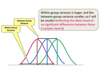
Within-Group
Variance
Between-Group
Variance
Between-group variance is large relative to the
within-group variance, so F statistic will be
larger & > critical value, therefore statistically
significant .
Conclusion – At least one of group means is
significantly different from other group means
Within-Group
Variance
Between-Group
Variance
Within-group variance is larger, and the
between-group variance smaller, so F will
be smaller (reflecting the likely-hood of
no significant differences between these
3 sample means)
Post-hoc Tests
• Used to determine which mean or group of means is/are
significantly different from the others (significant F)
• Depending upon research design & research question:
 Bonferroni (more powerful)
Only some pairs of sample means are to be tested
Desired alpha level is divided by no. of comparisons
 Tukey’s HSD Procedure
when all pairs of sample means are to be tested
 Scheffe’s Procedure (when sample sizes are unequal)
Application of ANOVA
• ANOVA is designed to detect differences among
means from populations subject to different treatments.
• ANOVA is a joint test, the equality of several
population means is tested simultaneously or jointly.
• ANOVA tests for the equality of several population
means by looking at two estimators of the population
variance (hence, analysis of variance).
Conclusion
• The one-way analysis of variance is used where there is a
single factor that will be set to three or more levels.
• t is not appropriate to analyse such data by repeated t-tests as
this will raise the risk of false positives above the acceptable
level of 5 per cent.
• If the ANOVA produces a significant result, this only tells us
that at least one level produces a different result from one of
the others.
• Follow-up tests needs to be carried out to find out which group
differs from each other.
THANK YOU

Shovan anova main

  • 1.
    One Way ANOVA Dr.Shovanpadhy, MBBS, MD DM 1st yr (Senior Resident) NIMS, Hyderabad
  • 2.
    Overview • Introduction. • WhyANOVA instead of multiple t-tests? • One way ANOVA. • Assumptions of One way ANOVA. • Steps in One way ANOVA. • Example. • Conclusion.
  • 3.
    Introduction • ANOVA isan abbreviation for the full name of the method: Analysis Of Variance. • Invented by R.A. Fisher in the 1918. • ANOVA is used to test the significance of the difference between more than two sample means. • Name “ANOVA” is a misnomer as it compares mean to check variance between group.
  • 4.
    Summary Table ofStatistical tests Level of Measurement Sample Characteristics Correlation 1 Sample 2 Sample K Sample (i.e., >2) Independent Dependent Independent Dependent Categorical or Nominal Χ2 or bi- nomina l Χ2 Macnarmar’s Χ2 Χ2 Cochran’s Q Rank or Ordinal Mann Whitney U Wilcoxin Matched Pairs Signed Ranks Kruskal Wallis H Friedman’s ANOVA Spearman’s rho Parametric (Interval & Ratio) z test or t test t test between groups t test within groups 1 way ANOVA between groups 1 way ANOVA (within or repeated measure) Pearson’s r Factorial (2 way) ANOVA Χ2
  • 5.
    Why ANOVA insteadof multiple t-tests? • If you are comparing means between more than two groups, we can choose two sample t-tests to compare the mean of one group with the mean of the other groups? :Before ANOVA, this was the only option available to compare means between more than two groups. • The problem with the multiple t-tests approach is that as the number of groups increases, the number of two sample t-tests also increases. • As the number of tests increases the probability of making a Type I error also increases.
  • 6.
    One way ANOVA •One way ANOVA (=F test) compares the mean of two or more group whenever there is one independent variable is involved. • It finds out whether there are any statistical significance difference between their group means. • If more then one independent variable is involved then it is called as N way ANOVA. • One way ANOVA specifically tests the null hypothesis. • H0 = u1 = u2 = u3 = uk , u = group mean & k= no. of groups. • If One way ANOVA shows a statistical significant result it means HA is true.
  • 7.
    Variables In Oneway ANOVA • In an ANOVA, there are two kinds of variables: independent and dependent • The independent variable is controlled or manipulated by the researcher. • It is a categorical (discrete) variable used to form the groupings of observations.
  • 8.
    • There aretwo types of independent variables: active and attribute. • If the independent variable is an active variable then we manipulate the values of the variable to study its affect on another variable. • For example, anxiety level is an active independent variable. • An attribute independent variable is a variable where we do not alter the variable during the study. • For example, we might want to study the effect of age on weight. We cannot change a person’s age, but we can study people of different ages and weights.
  • 9.
    • In theOne-way ANOVA, only one independent variable is considered, but there are two or more (theoretically any finite number) levels of the independent variable. • The independent variable is typically a categorical variable. • The independent variable (or factor) divides individuals into two or more groups or levels. • The procedure is a One-way ANOVA, since there is only one independent variable.
  • 10.
    • The (continuous)dependent variable is defined as the variable that is, or is presumed to be, the result of manipulating the independent variable. • In the One-way ANOVA, there is only one dependent variable – and hypotheses are formulated about the means of the groups on that dependent variable. • The dependent variable differentiates individuals on quantitative (continuous) dimension.
  • 11.
    Assumptions of Oneway ANOVA 1) All populations involved follow a normal distribution. 2) Homogeneity of variances: The variance within each group should be equal for all groups. 3) Independence of error: The error (variation of each value around its own group mean) should be independent for each value. 4) Only ONE independent variable should be checked whether it produces a significant difference between the groups.
  • 12.
    Example of Oneway ANOVA Group A Group B Group C 160,110,118,124,13 2 122,136,124,126,12 0,138 148,126,124,128,14 0 N1= 5 N2= 6 N3= 5 Mean=128.8 Mean= 127.66 Mean=133.2 EXAMPLE: A study conducted to assess & compare the effect of Treatment A vs Treatment B vs Treatment C on SBP in a specified population.
  • 13.
    ANOVA One way ANOVAThree way ANOVA Effect of Drugs on SBP Two way ANOVA Effect of Diet & Drugs on SBP Effect of Exercise, Drugs, Diet on SBP
  • 14.
    Steps in Oneway ANOVA 2. State Alpha 3. Calculate degrees of Freedom 4. Calculate test statistic - Calculate variance between samples - Calculate variance within the samples - Calculate F statistic 1. State null & alternative hypotheses
  • 15.
    Example- one wayANOVA Example: A investigator wants to find out the analgesic effect of aspirin vs diclofenac vs ibuprofen in a group of population with equal variances. Aspirin Diclofenac Ibuprofen 1 5 9 4 10 3 7 2 2 9 1 4 3 7 2
  • 16.
    Steps Involved 1.Null hypothesis– No significant difference in the means of 3 samples 2. State Alpha i.e 0.05 3. Calculate degrees of Freedom k-1 & n-k = 2 & 12 4. State decision rule Table value of F at 5% level of significance for d.f 2 & 12 is 3.88 The calculated value of F > 3.88 , H0 will be rejected 5. Calculate test statistic
  • 17.
    One way ANOVA:Table Source of Variation SS (Sum of Squares) Degrees of Freedom MS (Mean Square) Variance Ratio of F Between Samples SSB k-1 MSB= SSB/(k-1) MSB/MSW Within Samples SSW n-k MSW= SSW/(n-k) Total SS(Total) n-1
  • 18.
    Calculating variance BETWEENsamples 1. Calculate the mean of each sample. 2. Calculate the Grand mean. 3. Take the difference between means of various samples & grand average. 4. Square these deviations & obtain total which will give sum of squares between samples (SSC) 5. Divide the total obtained in step 4 by the degrees of freedom to calculate the mean sum of square between samples (MSC).
  • 19.
    Aspirin Diclofenac Ibuprofen 17 2 4 5 9 7 10 3 9 2 2 3 1 4 Total 24 M1= 4.8 25 M2 = 5 20 M3 = 4 4.8+ 5+ 4 3 Grand average = = 4.6
  • 20.
    Variance BETWEEN samples(M1=4.8, M2=5,M3=4) Sum of squares between samples (SSC) = n1 (M1 – Grand avg)2 + n2 (M2– Grand avg)2 + n3(M3– Grand avg)2 5 ( 4.8 - 4.6) 2 + 5 ( 5 - 4.8) 2 + 5 ( 4.6 - 4.8) 2 = 0.6 Calculation of Mean sum of squares between samples (MSB) =0.6/2 = 0.3 k= No of Samples, n= Total No of observations
  • 21.
    Calculating Variance WITHINSamples 1. Calculate mean value of each sample. 2. Take the deviations of the various items in a sample from the mean values of the respective samples. 3. Square these deviations & obtain total which gives the sum of square within the samples (SSE) 4. Divide the total obtained in 3rd step by the degrees of freedom to calculate the mean sum of squares within samples (MSE).
  • 22.
    Variance WITHIN samples(M1= 4.8, M2= 5,M3= 4) X1 (X1 – M1)2 X2 (X2– M2)2 X3 (X3– M3)2 1 14.4 7 4 2 4 4 0.64 5 0 9 25 7 4.84 10 25 3 1 9 17.64 2 9 2 4 3 3.24 1 16 4 0 40.76 54 34 Sum of squares within samples (SSE) = 40.76 + 54 +34 =128.76 Calculation of Mean Sum Of Squares within samples (MSW) = 128.76/12 = 10.73
  • 23.
    The mean sumof squares 1  k SSC MSC kn SSE MSE   Calculation of MSC- Mean sum of Squares between samples Calculation of MSE Mean Sum Of Squares within samples k= No of Samples, n= Total No of observations
  • 24.
    Calculation of Fstatsitics groupswithinyVariabilit groupsbetweenyVariabilit F  Compare the F-statistic value with F(critical) value which is obtained by looking for it in F distribution tables against degrees of freedom. The calculated value of F > table value H0 is rejected
  • 25.
    • F Value= MSB/MSW = 0.3/10.73 = 0.02. The Table value of F at 5% level of significance for d.f 2 & 12 is 3.88 The calculated value of F < table value H0 is accepted. Hence there no is significant difference in sample means
  • 26.
    Within-Group Variance Between-Group Variance Between-group variance islarge relative to the within-group variance, so F statistic will be larger & > critical value, therefore statistically significant . Conclusion – At least one of group means is significantly different from other group means
  • 27.
    Within-Group Variance Between-Group Variance Within-group variance islarger, and the between-group variance smaller, so F will be smaller (reflecting the likely-hood of no significant differences between these 3 sample means)
  • 28.
    Post-hoc Tests • Usedto determine which mean or group of means is/are significantly different from the others (significant F) • Depending upon research design & research question:  Bonferroni (more powerful) Only some pairs of sample means are to be tested Desired alpha level is divided by no. of comparisons  Tukey’s HSD Procedure when all pairs of sample means are to be tested  Scheffe’s Procedure (when sample sizes are unequal)
  • 29.
    Application of ANOVA •ANOVA is designed to detect differences among means from populations subject to different treatments. • ANOVA is a joint test, the equality of several population means is tested simultaneously or jointly. • ANOVA tests for the equality of several population means by looking at two estimators of the population variance (hence, analysis of variance).
  • 30.
    Conclusion • The one-wayanalysis of variance is used where there is a single factor that will be set to three or more levels. • t is not appropriate to analyse such data by repeated t-tests as this will raise the risk of false positives above the acceptable level of 5 per cent. • If the ANOVA produces a significant result, this only tells us that at least one level produces a different result from one of the others. • Follow-up tests needs to be carried out to find out which group differs from each other.
  • 31.