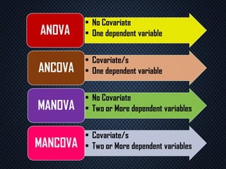
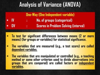
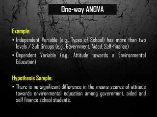
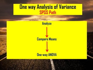
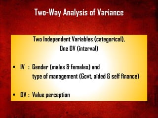
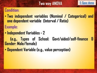
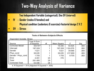
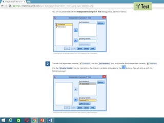
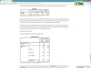
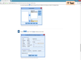
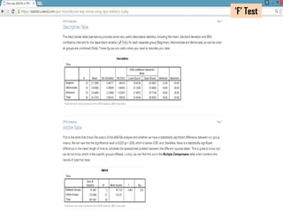
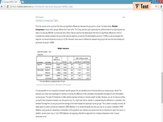
The document provides an overview of statistical methods including ANOVA, ANCOVA, MANOVA, and MANCOVA, focusing on their definitions, applications, and examples. It explains how these techniques are used to compare means across groups and the importance of controlling variables in experimental designs. SPSS is mentioned as a tool for conducting these analyses, with examples illustrating various scenarios and outcomes.

1. ANOVA
ANCOVA
MANOVA
&
MANCOVA
K.THIYAGU, Assistant Professor, Department of Education,
Central University of Kerala, Kasaragod

2. Learning Objectives
1. ANOVA
2. ANCOVA
3. MANOVA
4. MANCOVA
5. SPSS Help Desk

3. • No Covariate
• One dependent variableANOVA
• Covariate/s
• One dependent variableANCOVA
• No Covariate
• Two or More dependent variablesMANOVA
• Covariate/s
• Two or More dependent variablesMANCOVA

4. What is ANOVA?
✓ Statistical technique specially designed to test
whether the means of more than 2 quantitative
populations are equal.
✓ Developed by Sir Ronald A. Fisher in 1920’s.

5. Analysis of Variance (ANOVA)
▪ To test for significant differences between means (2 or more
means) (for groups or variables) for statistical significance.
▪ The variables that are measured (e.g., a test score) are called
dependent variables.
▪ The variables that are manipulated or controlled (e.g., a teaching
method or some other criterion used to divide observations into
groups that are compared) are called factors or independent
variables.
One-Way (One Independent variable)
▪ IV : No. of groups (categorical)
▪ DV : Scores in Problem Solving (interval)

6. One-way ANOVA
Example:
• Independent Variable (e.g., Types of School) has more than two
levels / Sub Groups (e.g., Government, Aided, Self-finance)
• Dependent Variable (e.g., Attitude towards a Environmental
Education)
Hypothesis Sample:
• There is no significant difference in the means scores of attitude
towards environmental education among government, aided and
self finance school students.

7. Within-Group
Variance
Between-Group
Variance
Between-group variance is large relative to the within-
group variance, so F statistic will be larger & > critical
value, therefore statistically significant .
Conclusion – At least one of group means is
significantly different from other group means

8. Within-Group
Variance
Between-Group
Variance
Within-group variance is larger, and the
between-group variance smaller, so F will be
smaller (reflecting the likely-hood of no
significant differences between these 3 sample
means)

9. One way ANOVA: Table
Source of
Variation
SS
(Sum of Squares)
Degrees of
Freedom
MS
(Mean Square)
Variance
Ratio of F
Between
Group
SSB k-1 MSB =
SSB /(k-1) F =
MSB/MSWWithin
Group
SSW n-k MSW=
SSW/(n-k)
Total SS(Total) n-1

10. Post-hoc Tests
• Used to determine which mean or group of means is/are significantly
different from the others (significant F)
• Depending upon research design & research question:
✓ Bonferroni (more powerful)
• Only some pairs of sample means are to be tested
• Desired alpha level is divided by no. of comparisons
✓ Tukey’s HSD Procedure
• when all pairs of sample means are to be tested
✓ Scheffe’s Procedure
• when sample sizes are unequal

11. Example of One-Way ANOVA
One-Way (One Independent variable)
▪ IV : No. of groups (categorical)
▪ DV : Scores in problem solving (interval)
ANOVA
Problem solving
216.600 2 108.300 93.124 .000
31.400 27 1.163
248.000 29
Between Groups
Within Groups
Total
Sum of
Squares df Mean Square F Sig.
Significant differences occur among the three groups on their problem solving scores,
F(2, 27) = 93.24, p<.001. The paired group significantly had the highest problem solving scores
(M=8.7)
Groups: Individuals=2.4, Pair=8.7, Group=3.9

12. Post ANOVA Measure
Multiple Comparisons
Dependent Variable: Problemsolving
-6.30000* .48228 .000 -7.4958 -5.1042
-1.50000* .48228 .012 -2.6958 -.3042
6.30000* .48228 .000 5.1042 7.4958
4.80000* .48228 .000 3.6042 5.9958
1.50000* .48228 .012 .3042 2.6958
-4.80000* .48228 .000 -5.9958 -3.6042
-6.30000* .48228 .000 -7.5491 -5.0509
-1.50000* .48228 .016 -2.7491 -.2509
6.30000* .48228 .000 5.0509 7.5491
4.80000* .48228 .000 3.5509 6.0491
1.50000* .48228 .016 .2509 2.7491
-4.80000* .48228 .000 -6.0491 -3.5509
(J) Groups
Pair
Group (3 members)
Individual
Group (3 members)
Individual
Pair
Pair
Group (3 members)
Individual
Group (3 members)
Individual
Pair
(I) Groups
Individual
Pair
Group (3 members)
Individual
Pair
Group (3 members)
Tukey HSD
Scheffe
Mean
Difference
(I-J) Std. Error Sig. Lower Bound Upper Bound
95% Confidence Interval
The mean difference is significant at the .05 level.*.

13. One way Analysis of Variance
SPSS Path
Analyze
Compare Means
One-way ANOVA

14. Two Way ANOVA

15. Two-Way Analysis of Variance
Two Independent Variables (categorical),
One DV (interval)
▪ IV : Gender (males & females) and
type of management (Govt, aided & self finance)
▪ DV : Value perception

16. Two way ANOVA
Condition:
• Two independent variables (Nominal / Categorical) and
one dependent variable (Interval / Ratio)
Example:
• Independent Variables - 2
(e.g., Types of School: Govt/aided/self-finance &
Gender: Male/female)
• Dependent Variable (e.g., value perception)
E-Spss demo

17. Two way ANOVA
Example
• Two independent factors- Management, Gender
• Dependent factor – value perception
Hypotheses Examples:
• Ho -Gender will have no significant effect on value perception
• Ho - Management will have no significant effect on value
perception
• Ho – Gender & Management interaction will have no significant
effect on value perception

18. Two-way ANOVA Table
Source of
Variation
Degrees of
Freedom
Sum of
Squares
Mean
Square
F-ratio P-value
Factor A r - 1 SSA MSA FA = MSA / MSE Tail area
Factor B c- 1 SSB MSB FB = MSB / MSE Tail area
Interaction (r – 1) (c – 1) SSAB MSAB FAB = MSAB / MSE Tail area
Error
(within)
rc(n – 1) SSE MSE
Total rcn - 1 SST

19. Two-Way Analysis of Variance
Two Independent Variable (categorical), One DV (interval)
▪ IV : Gender (males & females) and
Physical condition (sedentary & exercise)-factorial design 2 X 2
▪ DV : Stress
Tests of Between-Subjects Effects
Dependent Variable: Stress
48.916a 3 16.305 92.825 .000
197.539 1 197.539 1124.570 .000
7.021 1 7.021 39.969 .000
38.225 1 38.225 217.609 .000
1.705 1 1.705 9.705 .005
4.391 25 .176
261.490 29
53.308 28
Source
Corrected Model
Intercept
Gender
Phys_cond
Gender * Phys_cond
Error
Total
Corrected Total
Type III Sum
of Squares df Mean Square F Sig.
R Squared = .918 (Adjusted R Squared = .908)a.

20. Two-Way Analysis of Variance
SPSS Path
Analyze
General Linear Models
Univariate

21. Three way ANOVA

22. Three way ANOVA
Condition:
• Three independent variables and one dependent variable
Example:
• Independent Variables - 3
(e.g., Types of School: Govt/aided/self finance; Gender: Male/female &
Locality: Rural / Urban)
• Dependent Variable (e.g., Attitude about a Environmental Education)

23. Three-Way Analysis of Variance
SPSS Path
Analyze
General Linear Models
Univariate

24. ANOVA
One way ANOVA Three way ANOVA
Type of
Management on
EA
Two way ANOVA
Type of
Management,
Gender on EA
Type of Management,
Gender & Locality on
EA

25. ANCOVA

27. Analysis of Covariance (ANCOVA)
• "Controlling" for factors and how the inclusion of additional factors can
reduce the error SS and increase the statistical power (sensitivity) of our
design.
• This idea can be extended to continuous variables, and when such continuous
variables are included as factors in the design they are called covariates.
• Fixed covariates – In addition to the dependent variable we add other
measures of dependent variables.
• Changing covariates

28. ANCOVA with fixed covariates
• IV: Type of textbook,
• DV: Intelligence
• Covariate: Math ability
• By controlling the effect of textbook type on intelligence, we also
control its effect on math ability.

29. Tests of Between-Subjects Effects
Dependent Variable: Intelligence
5525.275a 2 2762.638 275.414 .000
281.123 1 281.123 28.026 .000
14.075 1 14.075 1.403 .252
260.426 1 260.426 25.962 .000
170.525 17 10.031
23576.000 20
5695.800 19
Source
Corrected Model
Intercept
math_ability
txtbook_type
Error
Total
Corrected Total
Type III Sum
of Squares df Mean Square F Sig.
R Squared = .970 (Adjusted R Squared = .967)a.
▪ Type of textbook significantly affects intelligence, p <.001. Students exposed to
textbook 1 had higher intelligence scores (M = 46.15) that those exposed to textbook 1
(M = 13.3).
▪ When the effects of textbook type on intelligence was controlled, textbook type do not
significantly vary on math ability (p =.252, n.s.).
▪ Math ability is not a covariate of intelligence on the effect of textbook type.

30. Tests of Within-Subjects Contrasts
Measure: MEASURE_1
137.269 1 137.269 50.069 .000
104.843 1 104.843 38.241 .000
90.976 1 90.976 33.184 .000
46.607 17 2.742
t2
Linear
Linear
Linear
Linear
Source
t2
t2 * math_ability
t2 * txtbook_type
Error(t2)
Type III Sum
of Squares df Mean Square F Sig.
Tests of Between-Subjects Effects
Measure: MEASURE_1
Transformed Variable: Average
217.757 1 217.757 45.090 .000
17.151 1 17.151 3.551 .077
118.502 1 118.502 24.538 .000
82.099 17 4.829
Source
Intercept
math_ability
txtbook_type
Error
Type III Sum
of Squares df Mean Square F Sig.

31. ANCOVA (Experimental Method)
When using a pre-post test research design, the Analysis of
Covariance allows a comparison of post-test scores with pre-
test scores factored out.
For example,
If comparing a experimental (treatment) and control group on
achievement motivation with a pre-post test design, the ANCOVA will
compare the treatment and control groups' post-test scores by
statistically setting the pre-test scores as being equal.

32. ANCOVA with changing covariates
• Applied for repeated measures
• When we have repeated measures, we are interested in testing the differences
in repeated measurements on the same subjects.
• We are actually interested in evaluating the significance of changes.
• If we have a covariate that is also measured at each point when the dependent
variable is measured, then we can compute the correlation between the changes
in the covariate and the changes in the dependent variable.
• For example, we could study math anxiety and math skills at the beginning and at
the end of the semester.
• It would be interesting to see whether any changes in math anxiety over the
semester correlate with changes in math skills.

33. Repeated
Measure
ANOVA

34. MANOVA
Multivariate Analysis of Variance

35. MANOVA
• MANOVA is used to test the significance of the effects of one or more IVs on
two or more DVs.
• It can be viewed as an extension of ANOVA with the key difference that we are
dealing with many dependent variables (not a single DV as in the case of
ANOVA)
Combination of dependent variables is called “joint distribution”
MANOVA gives answer to question
“ Is joint distribution of 2 or more DVs significantly related to one or more factors?”

36. • Dependent Variables ( at least 2)
• Interval /or ratio measurement scale
• May be correlated
• Multivariate normality
• Homogeneity of variance
• Independent Variables ( at least 1)
• Nominal measurement scale
• Each independent variable should be independent of each other

37. • The result of a MANOVA simply tells us that a difference exists (or not) across groups.
• It does not tell us which treatment(s) differ or what is contributing to the differences.
• For such information, we need to run ANOVAs with post hoc tests.
Various tests used-
✓Wilk's Lambda
➢ Widely used; good balance between power and assumptions
✓Pillai's Trace
➢ Useful when sample sizes are small, cell sizes are unequal, or covariances are not homogeneous
✓Hotelling's (Lawley-Hotelling) Trace
➢ Useful when examining differences between two groups

38. MANOVA
SPSS Path
Analyze
General Linear Model
Multivariate

39. SPSS Help Desk

40. https://statistics.laerd.com/

41. ‘t’ Test

42. ‘t’ Test

43. ‘t’ Test

44. ‘t’ Test

45. ‘t’ Test

46. ‘F’ Test

47. ‘F’ Test

48. ‘F’ Test

49. ‘F’ Test

50. ‘F’ Test

51. ‘F’ Test

52. ThankYou
Jai Bharat!
Acknowledgements
My teachers, My Guide , My Students
Source – Books / Images
Google