Reinforcement learning

1. Reinforcement
Learning
Ding Li 2021.3

2. Reinforcement Learning:
Learning from Interaction
Learn how to map situations to actions,
to maximize rewards.
The learner is not told which actions to take,
but instead must discover which actions yield
the most rewards by trying them.

3. 3
MULTI-ARMED BANDITS
How can an agent get as many rewards as
possible in limited time?
The rewards at each arm varies each time, but follows
a normal distribution, which is unknow to the agent
Epsilons Greedy: Balance of Exploration and Exploitation
10% probability (↋): randomly choosing an action (exploration)
90% probability (1-↋): taking the action with current maximum
reward (greedy, exploitation)
Estimated Average Reward after an action was chosen n times:
𝑄𝑛+1 =
𝑅1 + 𝑅2 + ⋯ + 𝑅𝑛
𝑛
= 𝑄𝑛 +
1
𝑛
𝑅𝑛 − 𝑄𝑛
Large ↋ learns fast
in the beginning
Final reward not high
due to exploration
Nonstationary Problem (the best arm changes over time) :
𝑄𝑛+1 = 𝑄𝑛 + 𝛼 𝑅𝑛 − 𝑄𝑛 𝛼: fixed step size
The new reward weights more than the old.
Weight of old reward decays exponentially.
Python code

4. 4
Agent: The leaner who interacts with Environment
State: Specific environment setting the agent is sensing
Action: What an agent can do to affect its state and generate reward
Policy: Map states to actions
Episode: agent and environment interact at time steps, t = 0, 1, 2, 3, ……, T (last time
step)
S0 S1
a0
S2
a1
S3
a2 a3
MDP: probability of St and Rt only depends on previous state and action.
MDP for Recycling Robot (state is battery level)
Return of step t for episodic task
Return of step t for continuous task
T is the terminal time step
r1 r2 r3 Policy 𝜋 𝑎|𝑠 : probability of taking action a at state s
deterministic: a is unique
stochastic: a is not unique
ST
…

5. 5
State-value function: expected return when starting in s and following
policy 𝜋
Action-value function: expected return when starting in s and taking action a
Gridworld: The cells of the grid correspond to the states of the environment. At each cell, four actions are possible:
north, south, east, and west. Actions that would take the agent out the grid leave its location unchanged, but also result in a reward
of −1. Other actions result in a reward of 0, except those that move the agent out of the special states A and B. γ = 0.9.
Bellman equation
Bellman optimality equation
Optimal Policies 𝜋∗: achieves the highest value possible in every state
Optimal state-value function 𝑣∗ 𝑠 = 𝑣𝜋∗
𝑠
Optimal action-value function

6. 6
Iterative policy evaluation (Bootstrapping):
Random initialization, continue the iteration until
converge
Policy Improvement (greedy policy):
Policy Iteration
Value Iteration (combine policy evaluation and policy
improvement)
Generalized Policy Iteration (GPI)
The general idea of letting
policy-evaluation and policy
improvement processes
interact, independent of the
granularity and other details
of the two processes
Asynchronous Dynamic Programming
A sweep of all states can be prohibitively expensive.
Asynchronous DP can update values of some states during one
sweep, and can focus on relevant states
Example of Policy
Iteration
Python code

7. 7
Estimate state values by averaging returns from experience
Estimate action values from experience
Exploring start: all state-action pairs might be selected as the start
Monte Carlo control
E: Monte Carlo estimation for q given current policy
I: Improve policy by taking greedy action
Blackjack
State: dealer’s card, player sum, usable ace? Action: Stick or Hit
ε-soft policy: exploration at each step, exploring start is not needed Target policy: the policy being learned, focus on exploitation (π)
Behavior policy: the policy generating behavior, focus on exploration (b)
Off policy learning: learning from behavior “off” the target policy (π≠b)
On policy learning: learning from behavior from the target policy (π=b)
Importance sampling ratio: relative probability of trajectories under π and b from t to T-1

8. 8
Update state value from next state value, only wait one step
TD error:
Example: Random Walk
TD converge
faster to lower
error than
Monty Carlo
Python code
Sarsa: On-policy TD Control (ε-greedy)
Q-learning: Off-policy TD Control
Expected Sarsa
More stable than Sarsa since it averages the action value of next state,
while Sarsa just uses the actual action of current run, with big randomness.
Off policy: it takes the best action from next state, not the real action taken.
On-policy algorithm can only learn from behaviors generated from current
policy. Data must be abandoned when policy updated. But any data can be
reused in off-policy algorithm, which is more sample efficient.
State-Action-Reward-State-Action

9. 9
Python code
Learn from previous experience
Improve learning efficiency

10. 10
Approximate value of a state s given weight vector w:
Typically, the number of weights is much less than the number of states.
Often μ(s) is chosen to be the fraction of time spent in s.
Mean Squared
Value Error
Stochastic gradient-descent (SGD): update w over time
Monti Carlo: use return value Gt to estimate 𝑣𝜋 𝑠
TD: use to estimate 𝑣𝜋 𝑠
Linear Methods
Corresponding to every state s, there is a real-valued
vector feature vector representing state s
At this TD fixed point

11. 11
Generalization: each tile covers significant state space
Discrimination: multiple tilings overlap each other
Episodic semi-gradient Sarsa: update W to
learn q
Consider the task of driving an underpowered car up
a steep mountain road. The difficulty is that gravity is
stronger than the car’s engine, and even at full
throttle the car cannot accelerate up the steep slope.
The only solution is to first move away from the goal
and up the opposite slope on the left. Then, by
applying full throttle the car can build up enough
inertia to carry it up the steep slope even though it is
slowing down the whole way.
Python code

12. 12
Average Reward: improve stabilization for continuous tasks
Return: difference between rewards and average
reward

13. 13
Neural Networks As Function
Approximation:
Raw
States
Transformed
States
Backpropagation is used to train the weights of the neural
networks.
Challenges:
• The input and output are not given in advance; but obtained through
interaction with environment.
• The representation of current state and future states are linked via neural
networks.
• The correct input is not available
• Feedback is often sparse
• Data generation and training process is coupled
• If function has sharp discontinuities.
Experience Replay:
An experience replay memory stores the k most recent experiences an
agent has gathered. If memory is full, the oldest experience is discarded to
make space for the latest one. Each time an agent trains, one or more
batches of data are sampled random-uniformly from the experience replay
memory. Each of these batches is used in turn to update the parameters of
the Q-function network.
Create
features
automaticall
y
1: Initialize learning rate α
2: Initialize τ
3: Initialize number of batches per training step, B
4: Initialize number of updates per batch, U
5: Initialize batch size N
6: Initialize experience replay memory with max size K
7: Randomly initialize the network parameters θ
8: for m = 1 . . . MAX_STEPS do
9: Gather and store h experiences (si,ai,ri,s′i) using the current policy
10: for b = 1 . . . B do
11: Sample a batch b of experiences from the experience replay memory
12: for u = 1 . . . U do
13: for i = 1 . . . N do
14: # Calculate target Q-values for each example
15: yi=ri+δs′iγ max a′i Qπθ(s′i,a′i) where δs′i=0 if s′i is terminal,
1 otherwise
16: end for
17: # Calculate the loss, for example using MSE
18: L(θ)=1N Σi(yi−Qπθ(si,ai))2
19: # Update the network’s parameters
20: θ = θ − α∇θL(θ)
21: end for
22: end for
23: Decay τ
24: end for
DQN Algorithm

14. 14
Target Networks
When the network parameters θ is updated to minimize
the difference between target value and calculated
value, the target value is also changed.
Target network is a second network with parameters φ which is a
lagged copy of θ. It reduces the changes in target value between
training steps.
Periodically, φ is updated to the current values of θ.
Double DQN
will be positively biased due to errors in each
=
DQN overestimates Qπ(s, a) for the (s, a) pairs that have been visited often.
The incorrect relative Q-values will be propagated backwards in time to
earlier (s, a) pairs and add error to those estimates as well. It is
therefore beneficial to reduce the overestimation of Q-values.
The training network θ is used to select the action.
The target network φ is used to evaluate that action.
Prioritized Experience Replay (PER)
Some experiences in the replay memory are more informative than others
ωi is the TD error for experience i, ε is a small positive number
priority for experience i
Experiment with Atari Game Pong
Double DQN + PER performs the best.
This is closely followed by DQN + PER, then Double DQN, and DQN.

15. 15
Ѳ: policy’s parameter vector, determine action from state
Parameter for action
value
Parameter for policy
Soft-max distribution
Policy parameterization has finer control on action than ε-
greedy
• Can autonomously decrease exploration over time.
• Fit stochastic application well (need action distribution)
• Sometime the policy is less complicated than the value function
The Policy Gradient Theorem for performance measure J

16. 16
Apply TD to REINFORCE Pendulum Swing Up
Tile-Coding Features
SoftMax Policy:
Early learning Final learning
Python code

17. 17
Foundations of Deep Reinforcement Learning

18. 18
Silver 2016

19. 19
Silver 2016
At each time step t of each simulation, an action at is
selected from state st
The bonus proportional to the prior probability but
decays with repeated visits to encourage exploration
The leaf node is evaluated by the value network vθ(sL) and the outcome zL of a
random rollout played out until terminal step T using the fast rollout policy pπ

20. 20
Silver 2017
• It is trained solely by self-play reinforcement learning, starting from
random play, without any supervision or use of human data.
• It uses only the black and white stones from the board as input features.
• It uses a single neural network, rather than separate policy and value
networks.
• It uses a simpler tree search that relies upon this single neural network
to evaluate positions and sample moves, without performing any Monte
Carlo rollouts.
• A new reinforcement learning algorithm was introduced that
incorporates lookahead search inside the training loop, resulting in rapid
improvement and precise and stable learning

21. 21
Silver 2017
The neural network (p, v)=fθ (s) is adjusted to minimize the error between the
predicted value v and the self-play winner z, and to maximize the similarity of
the neural network move probabilities p to the search probabilities π.

22. REINFORCEMENT
LEARNING
FRAMEWORKS
22

23. 23
Agents GitHub
TF-Agents makes implementing, deploying, and testing new Bandits and RL algorithms easier. It
provides well tested and modular components that can be modified and extended. It enables
fast code iteration, with good test integration and benchmarking.
Algorithms
• DQN: Human level control through deep reinforcement learning Mnih et al., 2015
• DDQN: Deep Reinforcement Learning with Double Q-learning Hasselt et al., 2015
• DDPG: Continuous control with deep reinforcement learning Lillicrap et al., 2015
• TD3: Addressing Function Approximation Error in Actor-Critic Methods Fujimoto et al., 2018
• REINFORCE: Simple Statistical Gradient-Following Algorithms for Connectionist Reinforcement
Learning Williams, 1992
• PPO: Proximal Policy Optimization Algorithms Schulman et al., 2017
• SAC: Soft Actor Critic Haarnoja et al., 2018
Tutorials
• Introduction to RL
• DQN

24. 24
RAY: Distributed Computing for ML
Researchers in UC Berkeley created the framework
To speed up ML training with CPU cores or cluster nodes
API in Python, core in C++
High level libraries use Ray internally for distributed computation
Ray GitHub
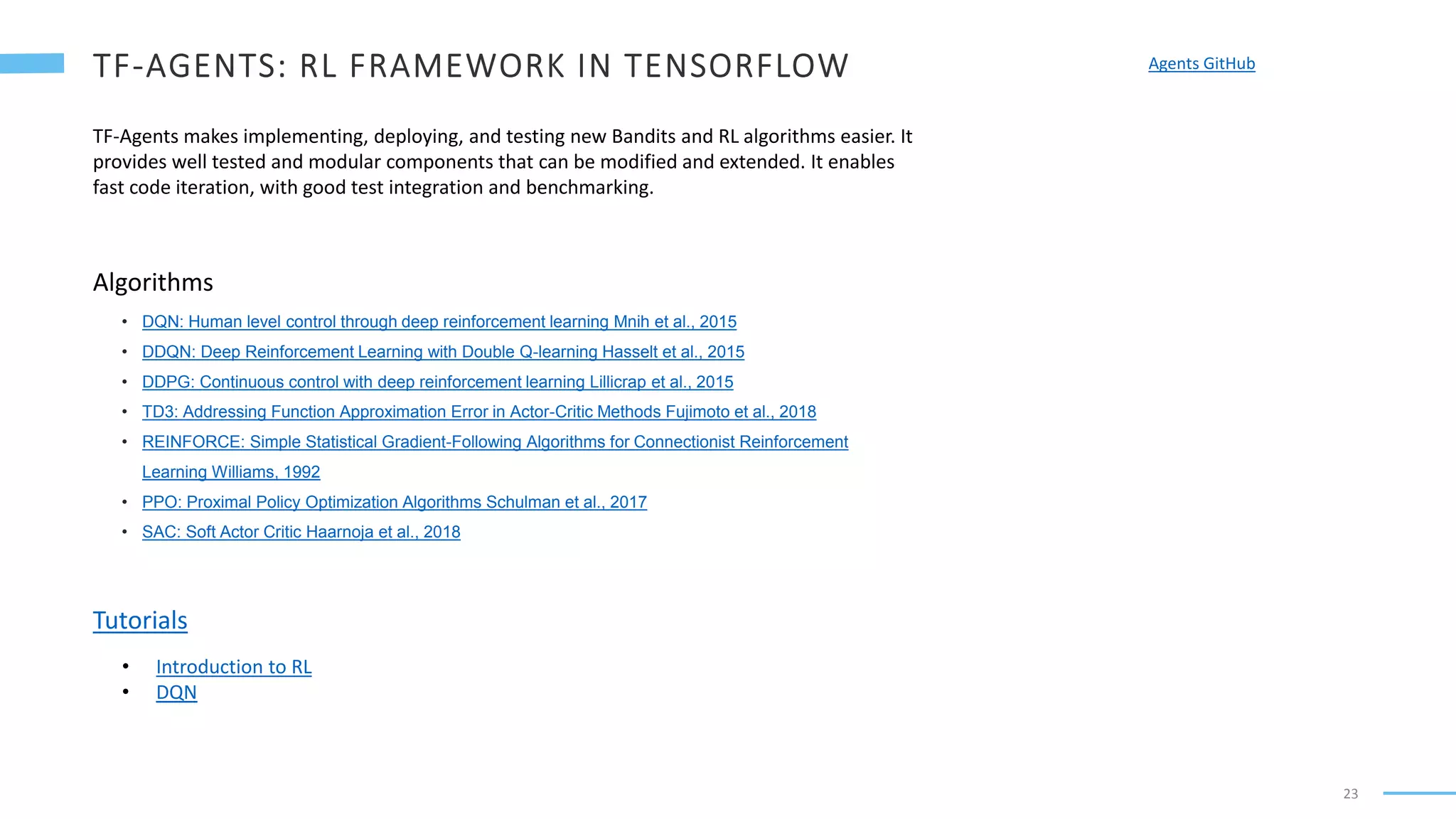
RlLib: Scalable Reinforcement Learning
import ray
import ray.rllib.agents.ppo as ppo
ray.init()
SELECT_ENV = "CartPole-v1"
config = ppo.DEFAULT_CONFIG.copy()
config['num_workers'] = 8
config['model']['fcnet_hiddens'] = [40,20]
trainer = ppo.PPOTrainer(config, SELECT_ENV)
for n in range(20):
result = trainer.train()
print(result['episode_reward_mean'])
Ray Tune: Hyperparameter Tuning
import ray
from ray import tune
ray.init()
tune.run(
"PPO",
stop={"episode_reward_mean": 400},
config={
"env": "CartPole-v1",
"num_gpus": 0,
"num_workers": 6,
"model": {
'fcnet_hiddens': [
tune.grid_search([20, 40, 60, 80]),
tune.grid_search([20, 40, 60, 80])]},},)

25. 25
Policy: calculate action from state
Colab RlLib
Environment
import gym
env = gym.make('CartPole-v0’)
# Choose an action (either 0 or 1).
def sample_policy(state):
return 0 if state[0] < 0 else 1
def rollout_policy(env, policy):
state = env.reset()
done = False
cumulative_reward = 0
while not done:
action = policy(state)
# Take the action in the environment.
state, reward, done, _ = env.step(action)
cumulative_reward += reward
return cumulative_reward
reward = rollout_policy(env, sample_policy)
import gym, ray
from ray.rllib.agents import ppo
class MyEnv(gym.Env):
def __init__(self, env_config):
self.action_space = <gym.Space>
self.observation_space = <gym.Space>
def reset(self):
return <obs>
def step(self, action):
return <obs>, <reward: float>, <done: bool>, <info: dict>
ray.init()
trainer = ppo.PPOTrainer(env=MyEnv, config={
"env_config": {}, # config to pass to env class
})
while True:
print(trainer.train())
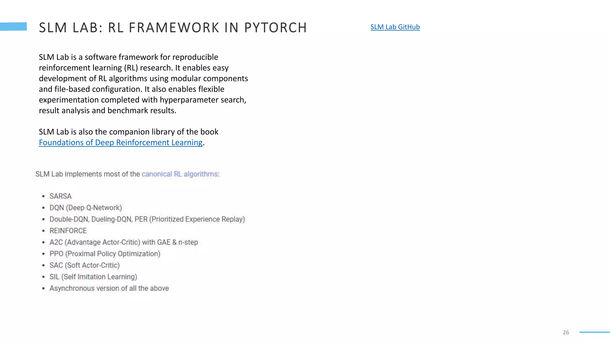
Algorithms

26. 26
SLM Lab GitHub
SLM Lab is a software framework for reproducible
reinforcement learning (RL) research. It enables easy
development of RL algorithms using modular components
and file-based configuration. It also enables flexible
experimentation completed with hyperparameter search,
result analysis and benchmark results.
SLM Lab is also the companion library of the book
Foundations of Deep Reinforcement Learning.

27. 27
A simple REINFORCE car pole spec file
1 #
slm_lab/spec/benchmark/reinforce/reinforce_cartpole.js
on
2
3 {
4 "reinforce_cartpole": {
5 "agent": [{
6 "name": "Reinforce",
7 "algorithm": {
8 "name": "Reinforce",
9 "action_pdtype": "default",
10 "action_policy": "default",
11 "center_return": true,
12 "explore_var_spec": null,
13 "gamma": 0.99,
14 "entropy_coef_spec": {
15 "name": "linear_decay",
16 "start_val": 0.01,
17 "end_val": 0.001,
18 "start_step": 0,
19 "end_step": 20000,
20 },
21 "training_frequency": 1
22 },
23 "memory": {
24 "name": "OnPolicyReplay"
25 },
26 "net": {
27 "type": "MLPNet",
28 "hid_layers": [64],
29 "hid_layers_activation": "selu",
30 "clip_grad_val": null,
31 "loss_spec": {
32 "name": "MSELoss"
33 },
34 "optim_spec": {
35 "name": "Adam",
36 "lr": 0.002
37 },
38 "lr_scheduler_spec": null
39 }
40 }],
41 "env": [{
42 "name": "CartPole-v0",
43 "max_t": null,
44 "max_frame": 100000,
45 }],
46 "body": {
47 "product": "outer",
48 "num": 1
49 },
50 "meta": {
51 "distributed": false,
52 "eval_frequency": 2000,
53 "max_session": 4,
54 "max_trial": 1,
55 },
56 ...
57 }
58 }
REINFORCE spec file with search spec for different gamma values
1 # slm_lab/spec/benchmark/reinforce/reinforce_cartpole.json
2
3 {
4 "reinforce_cartpole": {
5 ...
6 "meta": {
7 "distributed": false,
8 "eval_frequency": 2000,
9 "max_session": 4,
10 "max_trial": 1,
11 },
12 "search": {
13 "agent": [{
14 "algorithm": {
15 "gamma__grid_search": [0.1, 0.5, 0.7, 0.8, 0.90, 0.99, 0.999]
16 }
17 }]
18 }
19 }
20 }
γ values above 0.90 perform better,
with γ = 0.999 from trial 6 giving the
best result. When γ is too low, the
algorithm fails to learn a policy that
solves the problem, and the learning
curve stays flat.

28. 28
 Coursera
Reinforcement Learning Specialization
 Books
Reinforcement Learning, second edition: An Introduction
Foundations of Deep Reinforcement Learning
Hands-On Reinforcement Learning for Games
What Is Ray?