Reinforcement Learning
Tutorial
Peter Bodík
RAD Lab, UC Berkeley
Previous Lectures
• Supervised learning
– classification, regression
• Unsupervised learning
– clustering
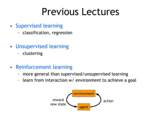
• Reinforcement learning
– more general than supervised/unsupervised learning
– learn from interaction w/ environment to achieve a goal
environment
agent
action
reward
new state
Today
• examples
• defining an RL problem
– Markov Decision Processes
• solving an RL problem
– Dynamic Programming
– Monte Carlo methods
– Temporal-Difference learning
Robot in a room
+1
-1
START
actions: UP, DOWN, LEFT, RIGHT
UP
80% move UP
10% move LEFT
10% move RIGHT
• reward +1 at [4,3], -1 at [4,2]
• reward -0.04 for each step
• what’s the strategy to achieve max reward?
• what if the actions were deterministic?
Other examples
• pole-balancing
• TD-Gammon [Gerry Tesauro]
• helicopter [Andrew Ng]
• no teacher who would say “good” or “bad”
– is reward “10” good or bad?
– rewards could be delayed
• similar to control theory
– more general, fewer constraints
• explore the environment and learn from experience
– not just blind search, try to be smart about it
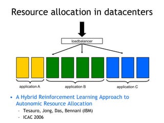
Resource allocation in datacenters
• A Hybrid Reinforcement Learning Approach to
Autonomic Resource Allocation
– Tesauro, Jong, Das, Bennani (IBM)
– ICAC 2006
loadbalancer
application A application B application C
Outline
• examples
• defining an RL problem
– Markov Decision Processes
• solving an RL problem
– Dynamic Programming
– Monte Carlo methods
– Temporal-Difference learning
Robot in a room
+1
-1
START
actions: UP, DOWN, LEFT, RIGHT
UP
80% move UP
10% move LEFT
10% move RIGHT
reward +1 at [4,3], -1 at [4,2]
reward -0.04 for each step
• states
• actions
• rewards
• what is the solution?
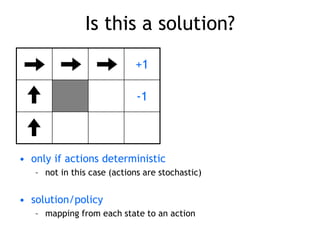
Is this a solution?
+1
-1
• only if actions deterministic
– not in this case (actions are stochastic)
• solution/policy
– mapping from each state to an action
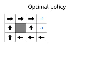
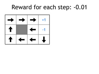
Optimal policy
+1
-1
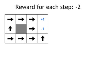
Reward for each step: -2
+1
-1
Reward for each step: -0.1
+1
-1
Reward for each step: -0.04
+1
-1
Reward for each step: -0.01
+1
-1
Reward for each step: +0.01
+1
-1
Markov Decision Process (MDP)
• set of states S, set of actions A, initial state S0
• transition model P(s,a,s’)
– P( [1,1], up, [1,2] ) = 0.8
• reward function r(s)
– r( [4,3] ) = +1
• goal: maximize cumulative reward in the long run
• policy: mapping from S to A
– (s) or (s,a) (deterministic vs. stochastic)
• reinforcement learning
– transitions and rewards usually not available
– how to change the policy based on experience
– how to explore the environment
environment
agent
action
reward
new state
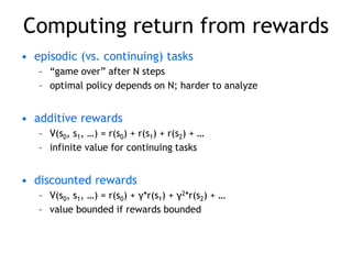
Computing return from rewards
• episodic (vs. continuing) tasks
– “game over” after N steps
– optimal policy depends on N; harder to analyze
• additive rewards
– V(s0, s1, …) = r(s0) + r(s1) + r(s2) + …
– infinite value for continuing tasks
• discounted rewards
– V(s0, s1, …) = r(s0) + γ*r(s1) + γ2*r(s2) + …
– value bounded if rewards bounded
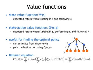
Value functions
• state value function: V(s)
– expected return when starting in s and following 
• state-action value function: Q(s,a)
– expected return when starting in s, performing a, and following 
• useful for finding the optimal policy
– can estimate from experience
– pick the best action using Q(s,a)
• Bellman equation
s
a
s’
r
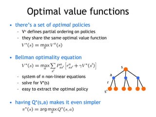
Optimal value functions
• there’s a set of optimal policies
– V defines partial ordering on policies
– they share the same optimal value function
• Bellman optimality equation
– system of n non-linear equations
– solve for V*(s)
– easy to extract the optimal policy
• having Q*(s,a) makes it even simpler
s
a
s’
r
Outline
• examples
• defining an RL problem
– Markov Decision Processes
• solving an RL problem
– Dynamic Programming
– Monte Carlo methods
– Temporal-Difference learning
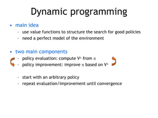
Dynamic programming
• main idea
– use value functions to structure the search for good policies
– need a perfect model of the environment
• two main components
– policy evaluation: compute V from 
– policy improvement: improve  based on V
– start with an arbitrary policy
– repeat evaluation/improvement until convergence
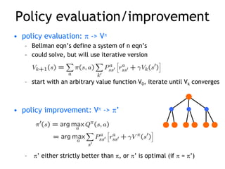
Policy evaluation/improvement
• policy evaluation:  -> V
– Bellman eqn’s define a system of n eqn’s
– could solve, but will use iterative version
– start with an arbitrary value function V0, iterate until Vk converges
• policy improvement: V -> ’
– ’ either strictly better than , or ’ is optimal (if  = ’)
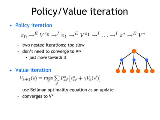
Policy/Value iteration
• Policy iteration
– two nested iterations; too slow
– don’t need to converge to Vk
• just move towards it
• Value iteration
– use Bellman optimality equation as an update
– converges to V*
Using DP
• need complete model of the environment and rewards
– robot in a room
• state space, action space, transition model
• can we use DP to solve
– robot in a room?
– back gammon?
– helicopter?
Outline
• examples
• defining an RL problem
– Markov Decision Processes
• solving an RL problem
– Dynamic Programming
– Monte Carlo methods
– Temporal-Difference learning
• miscellaneous
– state representation
– function approximation
– rewards
Monte Carlo methods
• don’t need full knowledge of environment
– just experience, or
– simulated experience
• but similar to DP
– policy evaluation, policy improvement
• averaging sample returns
– defined only for episodic tasks
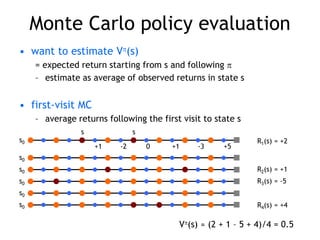
Monte Carlo policy evaluation
• want to estimate V(s)
= expected return starting from s and following 
– estimate as average of observed returns in state s
• first-visit MC
– average returns following the first visit to state s
s0
s s
+1 -2 0 +1 -3 +5
R1(s) = +2
s0
s0
s0
s0
s0
R2(s) = +1
R3(s) = -5
R4(s) = +4
V(s) ≈ (2 + 1 – 5 + 4)/4 = 0.5
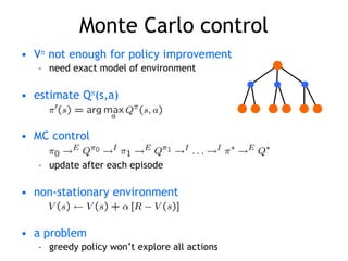
Monte Carlo control
• V not enough for policy improvement
– need exact model of environment
• estimate Q(s,a)
• MC control
– update after each episode
• non-stationary environment
• a problem
– greedy policy won’t explore all actions
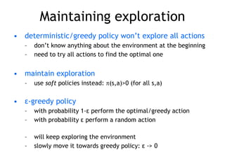
Maintaining exploration
• deterministic/greedy policy won’t explore all actions
– don’t know anything about the environment at the beginning
– need to try all actions to find the optimal one
• maintain exploration
– use soft policies instead: (s,a)>0 (for all s,a)
• ε-greedy policy
– with probability 1-ε perform the optimal/greedy action
– with probability ε perform a random action
– will keep exploring the environment
– slowly move it towards greedy policy: ε -> 0
Simulated experience
• 5-card draw poker
– s0: A, A, 6, A, 2
– a0: discard 6, 2
– s1: A, A, A, A, 9 + dealer takes 4 cards
– return: +1 (probably)
• DP
– list all states, actions, compute P(s,a,s’)
• P( [A,A,6,A,2], [6,2], [A,9,4] ) = 0.00192
• MC
– all you need are sample episodes
– let MC play against a random policy, or itself, or another
algorithm
Summary of Monte Carlo
• don’t need model of environment
– averaging of sample returns
– only for episodic tasks
• learn from sample episodes or simulated experience
• can concentrate on “important” states
– don’t need a full sweep
• need to maintain exploration
– use soft policies
Outline
• examples
• defining an RL problem
– Markov Decision Processes
• solving an RL problem
– Dynamic Programming
– Monte Carlo methods
– Temporal-Difference learning
• miscellaneous
– state representation
– function approximation
– rewards
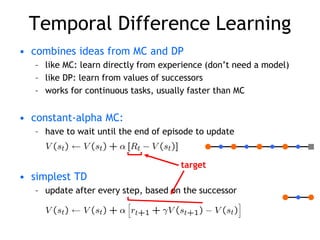
Temporal Difference Learning
• combines ideas from MC and DP
– like MC: learn directly from experience (don’t need a model)
– like DP: learn from values of successors
– works for continuous tasks, usually faster than MC
• constant-alpha MC:
– have to wait until the end of episode to update
• simplest TD
– update after every step, based on the successor
target
MC vs. TD
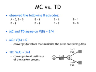
• observed the following 8 episodes:
A – 0, B – 0 B – 1 B – 1 B - 1
B – 1 B – 1 B – 1 B – 0
• MC and TD agree on V(B) = 3/4
• MC: V(A) = 0
– converges to values that minimize the error on training data
• TD: V(A) = 3/4
– converges to ML estimate
of the Markov process
A B
r = 0
100%
r = 1
75%
r = 0
25%
Sarsa
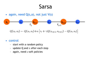
• again, need Q(s,a), not just V(s)
• control
– start with a random policy
– update Q and  after each step
– again, need -soft policies
st st+1
at st+2
at+1 at+2
rt rt+1
The RL Intro book
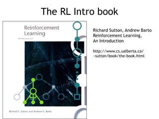
Richard Sutton, Andrew Barto
Reinforcement Learning,
An Introduction
http://www.cs.ualberta.ca/
~sutton/book/the-book.html
Backup slides
Q-learning
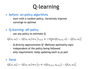
• before: on-policy algorithms
– start with a random policy, iteratively improve
– converge to optimal
• Q-learning: off-policy
– use any policy to estimate Q
– Q directly approximates Q* (Bellman optimality eqn)
– independent of the policy being followed
– only requirement: keep updating each (s,a) pair
• Sarsa
Outline
• examples
• defining an RL problem
– Markov Decision Processes
• solving an RL problem
– Dynamic Programming
– Monte Carlo methods
– Temporal-Difference learning
• miscellaneous
– state representation
– function approximation
– rewards
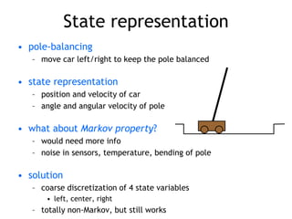
State representation
• pole-balancing
– move car left/right to keep the pole balanced
• state representation
– position and velocity of car
– angle and angular velocity of pole
• what about Markov property?
– would need more info
– noise in sensors, temperature, bending of pole
• solution
– coarse discretization of 4 state variables
• left, center, right
– totally non-Markov, but still works
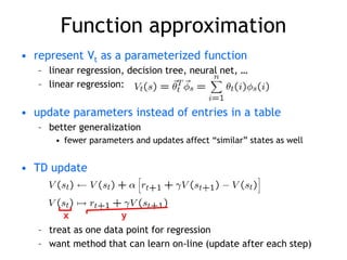
Function approximation
• represent Vt as a parameterized function
– linear regression, decision tree, neural net, …
– linear regression:
• update parameters instead of entries in a table
– better generalization
• fewer parameters and updates affect “similar” states as well
• TD update
– treat as one data point for regression
– want method that can learn on-line (update after each step)
x y
Features
• tile coding, coarse coding
– binary features
• radial basis functions
– typically a Gaussian
– between 0 and 1
[ Sutton & Barto, Reinforcement Learning ]
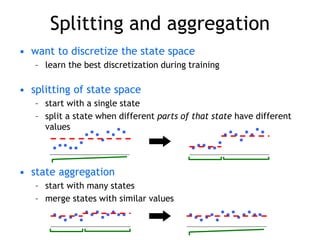
Splitting and aggregation
• want to discretize the state space
– learn the best discretization during training
• splitting of state space
– start with a single state
– split a state when different parts of that state have different
values
• state aggregation
– start with many states
– merge states with similar values
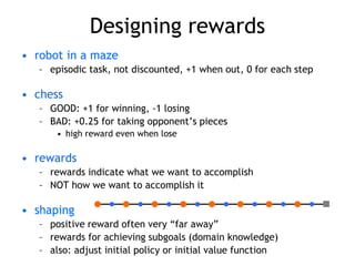
Designing rewards
• robot in a maze
– episodic task, not discounted, +1 when out, 0 for each step
• chess
– GOOD: +1 for winning, -1 losing
– BAD: +0.25 for taking opponent’s pieces
• high reward even when lose
• rewards
– rewards indicate what we want to accomplish
– NOT how we want to accomplish it
• shaping
– positive reward often very “far away”
– rewards for achieving subgoals (domain knowledge)
– also: adjust initial policy or initial value function
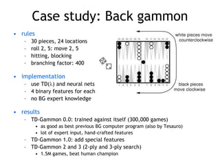
Case study: Back gammon
• rules
– 30 pieces, 24 locations
– roll 2, 5: move 2, 5
– hitting, blocking
– branching factor: 400
• implementation
– use TD() and neural nets
– 4 binary features for each position on board (# white pieces)
– no BG expert knowledge
• results
– TD-Gammon 0.0: trained against itself (300,000 games)
• as good as best previous BG computer program (also by Tesauro)
• lot of expert input, hand-crafted features
– TD-Gammon 1.0: add special features
– TD-Gammon 2 and 3 (2-ply and 3-ply search)
• 1.5M games, beat human champion
Summary
• Reinforcement learning
– use when need to make decisions in uncertain environment
• solution methods
– dynamic programming
• need complete model
– Monte Carlo
– time-difference learning (Sarsa, Q-learning)
• most work
– algorithms simple
– need to design features, state representation, rewards

reinforcement-learning.prsentation for c

  • 1.
  • 2.
    Previous Lectures • Supervisedlearning – classification, regression • Unsupervised learning – clustering • Reinforcement learning – more general than supervised/unsupervised learning – learn from interaction w/ environment to achieve a goal environment agent action reward new state
  • 3.
    Today • examples • definingan RL problem – Markov Decision Processes • solving an RL problem – Dynamic Programming – Monte Carlo methods – Temporal-Difference learning
  • 4.
    Robot in aroom +1 -1 START actions: UP, DOWN, LEFT, RIGHT UP 80% move UP 10% move LEFT 10% move RIGHT • reward +1 at [4,3], -1 at [4,2] • reward -0.04 for each step • what’s the strategy to achieve max reward? • what if the actions were deterministic?
  • 5.
    Other examples • pole-balancing •TD-Gammon [Gerry Tesauro] • helicopter [Andrew Ng] • no teacher who would say “good” or “bad” – is reward “10” good or bad? – rewards could be delayed • similar to control theory – more general, fewer constraints • explore the environment and learn from experience – not just blind search, try to be smart about it
  • 6.
    Resource allocation indatacenters • A Hybrid Reinforcement Learning Approach to Autonomic Resource Allocation – Tesauro, Jong, Das, Bennani (IBM) – ICAC 2006 loadbalancer application A application B application C
  • 7.
    Outline • examples • definingan RL problem – Markov Decision Processes • solving an RL problem – Dynamic Programming – Monte Carlo methods – Temporal-Difference learning
  • 8.
    Robot in aroom +1 -1 START actions: UP, DOWN, LEFT, RIGHT UP 80% move UP 10% move LEFT 10% move RIGHT reward +1 at [4,3], -1 at [4,2] reward -0.04 for each step • states • actions • rewards • what is the solution?
  • 9.
    Is this asolution? +1 -1 • only if actions deterministic – not in this case (actions are stochastic) • solution/policy – mapping from each state to an action
  • 10.
  • 11.
    Reward for eachstep: -2 +1 -1
  • 12.
    Reward for eachstep: -0.1 +1 -1
  • 13.
    Reward for eachstep: -0.04 +1 -1
  • 14.
    Reward for eachstep: -0.01 +1 -1
  • 15.
    Reward for eachstep: +0.01 +1 -1
  • 16.
    Markov Decision Process(MDP) • set of states S, set of actions A, initial state S0 • transition model P(s,a,s’) – P( [1,1], up, [1,2] ) = 0.8 • reward function r(s) – r( [4,3] ) = +1 • goal: maximize cumulative reward in the long run • policy: mapping from S to A – (s) or (s,a) (deterministic vs. stochastic) • reinforcement learning – transitions and rewards usually not available – how to change the policy based on experience – how to explore the environment environment agent action reward new state
  • 17.
    Computing return fromrewards • episodic (vs. continuing) tasks – “game over” after N steps – optimal policy depends on N; harder to analyze • additive rewards – V(s0, s1, …) = r(s0) + r(s1) + r(s2) + … – infinite value for continuing tasks • discounted rewards – V(s0, s1, …) = r(s0) + γ*r(s1) + γ2*r(s2) + … – value bounded if rewards bounded
  • 18.
    Value functions • statevalue function: V(s) – expected return when starting in s and following  • state-action value function: Q(s,a) – expected return when starting in s, performing a, and following  • useful for finding the optimal policy – can estimate from experience – pick the best action using Q(s,a) • Bellman equation s a s’ r
  • 19.
    Optimal value functions •there’s a set of optimal policies – V defines partial ordering on policies – they share the same optimal value function • Bellman optimality equation – system of n non-linear equations – solve for V*(s) – easy to extract the optimal policy • having Q*(s,a) makes it even simpler s a s’ r
  • 20.
    Outline • examples • definingan RL problem – Markov Decision Processes • solving an RL problem – Dynamic Programming – Monte Carlo methods – Temporal-Difference learning
  • 21.
    Dynamic programming • mainidea – use value functions to structure the search for good policies – need a perfect model of the environment • two main components – policy evaluation: compute V from  – policy improvement: improve  based on V – start with an arbitrary policy – repeat evaluation/improvement until convergence
  • 22.
    Policy evaluation/improvement • policyevaluation:  -> V – Bellman eqn’s define a system of n eqn’s – could solve, but will use iterative version – start with an arbitrary value function V0, iterate until Vk converges • policy improvement: V -> ’ – ’ either strictly better than , or ’ is optimal (if  = ’)
  • 23.
    Policy/Value iteration • Policyiteration – two nested iterations; too slow – don’t need to converge to Vk • just move towards it • Value iteration – use Bellman optimality equation as an update – converges to V*
  • 24.
    Using DP • needcomplete model of the environment and rewards – robot in a room • state space, action space, transition model • can we use DP to solve – robot in a room? – back gammon? – helicopter?
  • 25.
    Outline • examples • definingan RL problem – Markov Decision Processes • solving an RL problem – Dynamic Programming – Monte Carlo methods – Temporal-Difference learning • miscellaneous – state representation – function approximation – rewards
  • 26.
    Monte Carlo methods •don’t need full knowledge of environment – just experience, or – simulated experience • but similar to DP – policy evaluation, policy improvement • averaging sample returns – defined only for episodic tasks
  • 27.
    Monte Carlo policyevaluation • want to estimate V(s) = expected return starting from s and following  – estimate as average of observed returns in state s • first-visit MC – average returns following the first visit to state s s0 s s +1 -2 0 +1 -3 +5 R1(s) = +2 s0 s0 s0 s0 s0 R2(s) = +1 R3(s) = -5 R4(s) = +4 V(s) ≈ (2 + 1 – 5 + 4)/4 = 0.5
  • 28.
    Monte Carlo control •V not enough for policy improvement – need exact model of environment • estimate Q(s,a) • MC control – update after each episode • non-stationary environment • a problem – greedy policy won’t explore all actions
  • 29.
    Maintaining exploration • deterministic/greedypolicy won’t explore all actions – don’t know anything about the environment at the beginning – need to try all actions to find the optimal one • maintain exploration – use soft policies instead: (s,a)>0 (for all s,a) • ε-greedy policy – with probability 1-ε perform the optimal/greedy action – with probability ε perform a random action – will keep exploring the environment – slowly move it towards greedy policy: ε -> 0
  • 30.
    Simulated experience • 5-carddraw poker – s0: A, A, 6, A, 2 – a0: discard 6, 2 – s1: A, A, A, A, 9 + dealer takes 4 cards – return: +1 (probably) • DP – list all states, actions, compute P(s,a,s’) • P( [A,A,6,A,2], [6,2], [A,9,4] ) = 0.00192 • MC – all you need are sample episodes – let MC play against a random policy, or itself, or another algorithm
  • 31.
    Summary of MonteCarlo • don’t need model of environment – averaging of sample returns – only for episodic tasks • learn from sample episodes or simulated experience • can concentrate on “important” states – don’t need a full sweep • need to maintain exploration – use soft policies
  • 32.
    Outline • examples • definingan RL problem – Markov Decision Processes • solving an RL problem – Dynamic Programming – Monte Carlo methods – Temporal-Difference learning • miscellaneous – state representation – function approximation – rewards
  • 33.
    Temporal Difference Learning •combines ideas from MC and DP – like MC: learn directly from experience (don’t need a model) – like DP: learn from values of successors – works for continuous tasks, usually faster than MC • constant-alpha MC: – have to wait until the end of episode to update • simplest TD – update after every step, based on the successor target
  • 34.
    MC vs. TD •observed the following 8 episodes: A – 0, B – 0 B – 1 B – 1 B - 1 B – 1 B – 1 B – 1 B – 0 • MC and TD agree on V(B) = 3/4 • MC: V(A) = 0 – converges to values that minimize the error on training data • TD: V(A) = 3/4 – converges to ML estimate of the Markov process A B r = 0 100% r = 1 75% r = 0 25%
  • 35.
    Sarsa • again, needQ(s,a), not just V(s) • control – start with a random policy – update Q and  after each step – again, need -soft policies st st+1 at st+2 at+1 at+2 rt rt+1
  • 36.
    The RL Introbook Richard Sutton, Andrew Barto Reinforcement Learning, An Introduction http://www.cs.ualberta.ca/ ~sutton/book/the-book.html
  • 37.
  • 38.
    Q-learning • before: on-policyalgorithms – start with a random policy, iteratively improve – converge to optimal • Q-learning: off-policy – use any policy to estimate Q – Q directly approximates Q* (Bellman optimality eqn) – independent of the policy being followed – only requirement: keep updating each (s,a) pair • Sarsa
  • 39.
    Outline • examples • definingan RL problem – Markov Decision Processes • solving an RL problem – Dynamic Programming – Monte Carlo methods – Temporal-Difference learning • miscellaneous – state representation – function approximation – rewards
  • 40.
    State representation • pole-balancing –move car left/right to keep the pole balanced • state representation – position and velocity of car – angle and angular velocity of pole • what about Markov property? – would need more info – noise in sensors, temperature, bending of pole • solution – coarse discretization of 4 state variables • left, center, right – totally non-Markov, but still works
  • 41.
    Function approximation • representVt as a parameterized function – linear regression, decision tree, neural net, … – linear regression: • update parameters instead of entries in a table – better generalization • fewer parameters and updates affect “similar” states as well • TD update – treat as one data point for regression – want method that can learn on-line (update after each step) x y
  • 42.
    Features • tile coding,coarse coding – binary features • radial basis functions – typically a Gaussian – between 0 and 1 [ Sutton & Barto, Reinforcement Learning ]
  • 43.
    Splitting and aggregation •want to discretize the state space – learn the best discretization during training • splitting of state space – start with a single state – split a state when different parts of that state have different values • state aggregation – start with many states – merge states with similar values
  • 44.
    Designing rewards • robotin a maze – episodic task, not discounted, +1 when out, 0 for each step • chess – GOOD: +1 for winning, -1 losing – BAD: +0.25 for taking opponent’s pieces • high reward even when lose • rewards – rewards indicate what we want to accomplish – NOT how we want to accomplish it • shaping – positive reward often very “far away” – rewards for achieving subgoals (domain knowledge) – also: adjust initial policy or initial value function
  • 45.
    Case study: Backgammon • rules – 30 pieces, 24 locations – roll 2, 5: move 2, 5 – hitting, blocking – branching factor: 400 • implementation – use TD() and neural nets – 4 binary features for each position on board (# white pieces) – no BG expert knowledge • results – TD-Gammon 0.0: trained against itself (300,000 games) • as good as best previous BG computer program (also by Tesauro) • lot of expert input, hand-crafted features – TD-Gammon 1.0: add special features – TD-Gammon 2 and 3 (2-ply and 3-ply search) • 1.5M games, beat human champion
  • 46.
    Summary • Reinforcement learning –use when need to make decisions in uncertain environment • solution methods – dynamic programming • need complete model – Monte Carlo – time-difference learning (Sarsa, Q-learning) • most work – algorithms simple – need to design features, state representation, rewards