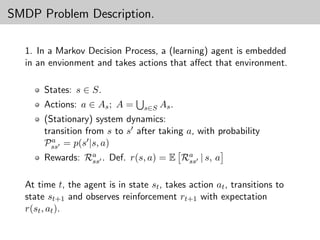
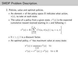
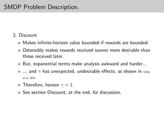
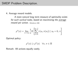
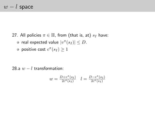
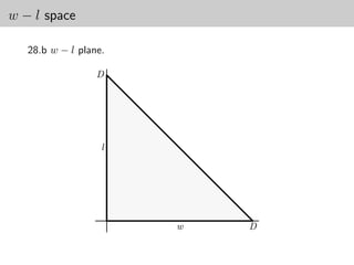
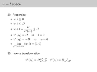
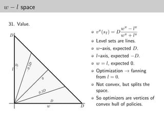
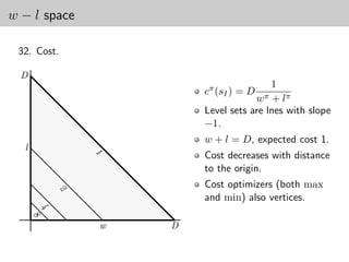
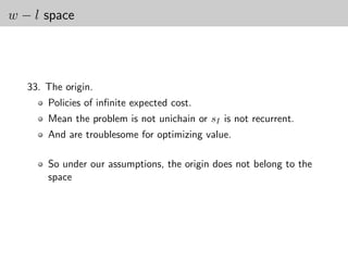
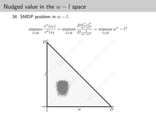
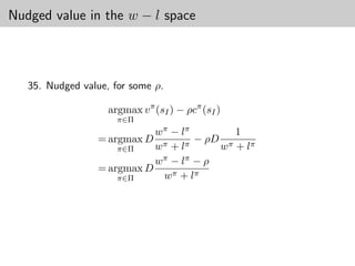
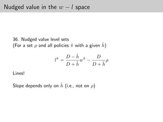
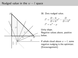
The document provides a summary of Semi-Markov Decision Processes (SMDPs) in 10 points:
1. It describes the basic components of an SMDP including states, actions, rewards, policies, and value functions.
2. It discusses the concepts of optimal policies, average reward models, and discount factors in SMDPs.
3. It introduces the idea of transition times in SMDPs, which allows actions to take varying amounts of time. This makes SMDPs a generalization of Markov Decision Processes.
4. It notes that algorithms for solving SMDPs typically involve estimating the average reward per action to find an optimal policy.


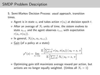
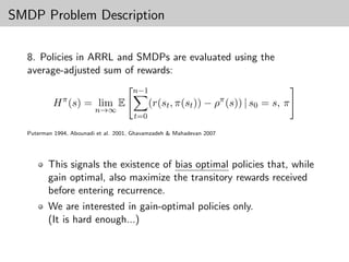

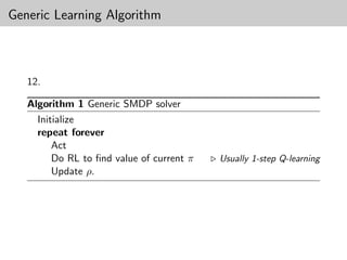
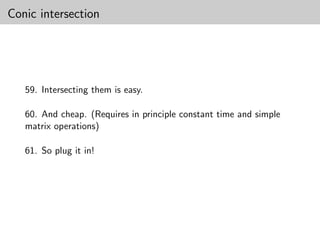
![SSP Q-Learning
15. Stochastic Shortest Path Q-Learning
Most interesting. ARRL
If unichain and exists s recurrent (Assumption 2.1 ):
ˆ
SSP Q-learning is based on the observation that
the average cost under any stationary policy is
simply the ratio of expected total cost and expected
time between two successive visits to the reference
state [ˆ]
s
Thus, they propose (after Bertsekas 1998) making the process
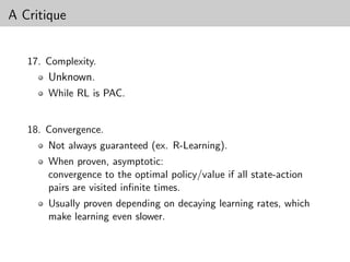
episodic, splitting s into the (unique) initial and terminal
ˆ
states.
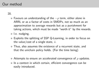
If the Assumption holds, termination has probability 1.
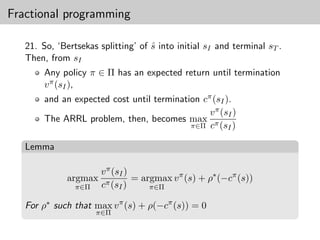
Only the value/cost of the initial state are important.
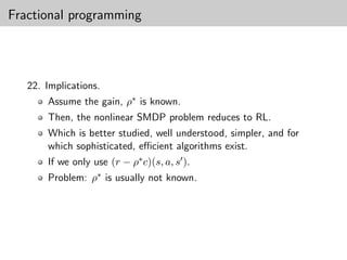
Optimal solution “can be shown to happen” when H(ˆ) = 0.
s
(See next section)](https://image.slidesharecdn.com/pres-130417151613-phpapp02/85/100-things-I-know-19-320.jpg)
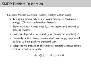
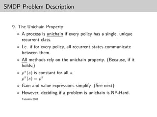
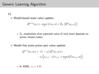
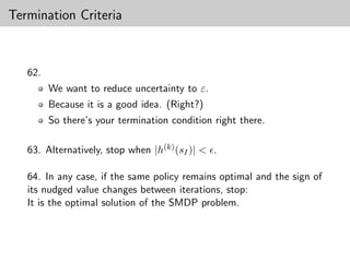
![SSP Q-Learning
16. SSPQ ρ update.
ρt+1 ← ρt + αt min Qt (ˆ, a),
s
a
where
2
αt → ∞; αt < ∞.
t t
But it is hard to prove boundedness of {ρt }, so suggested instead
ρt+1 ← Γ ρt + αt min Qt (ˆ, a) ,
s
a
with Γ(·) a projection to [−K, K] and ρ∗ ∈ (−K, K).](https://image.slidesharecdn.com/pres-130417151613-phpapp02/85/100-things-I-know-20-320.jpg)
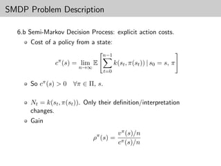
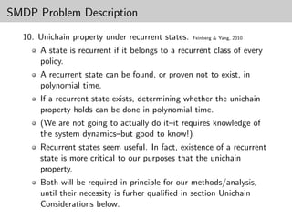
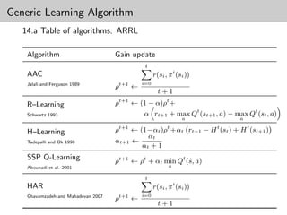
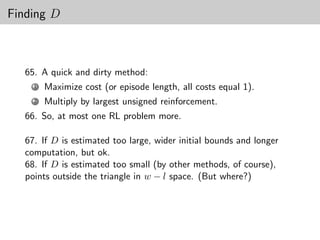
![A Critique
19. Convergence of ρ updates.
... while the second “slow” iteration gradually guides
[ρt ] to the desired value.
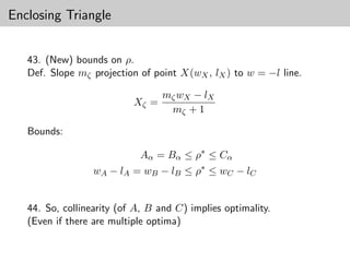
Abounadi et al. 2001
It is the slow one!
Must be so for sufficient approximation of current policy value
for improvement.
Initially biased towards (likely poor) observed returns at the
start.
A long time must probably pass following the optimal policy
for ρ to converge to actual value.](https://image.slidesharecdn.com/pres-130417151613-phpapp02/85/100-things-I-know-22-320.jpg)


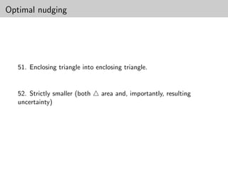


![Lecture on nk [compatibility mode]](https://cdn.slidesharecdn.com/ss_thumbnails/lectureonnkcompatibilitymode-110825092241-phpapp01-thumbnail.jpg?width=640&height=640&fit=bounds)