Machine learning (13)

CS229 Lecture notes
Andrew Ng
Part XIII
Reinforcement Learning and
Control
We now begin our study of reinforcement learning and adaptive control.
In supervised learning, we saw algorithms that tried to make their outputs
mimic the labels y given in the training set. In that setting, the labels gave
an unambiguous “right answer” for each of the inputs x. In contrast, for
many sequential decision making and control problems, it is very difficult to
provide this type of explicit supervision to a learning algorithm. For example,
if we have just built a four-legged robot and are trying to program it to walk,
then initially we have no idea what the “correct” actions to take are to make
it walk, and so do not know how to provide explicit supervision for a learning
algorithm to try to mimic.
In the reinforcement learning framework, we will instead provide our al-
gorithms only a reward function, which indicates to the learning agent when
it is doing well, and when it is doing poorly. In the four-legged walking ex-
ample, the reward function might give the robot positive rewards for moving
forwards, and negative rewards for either moving backwards or falling over.
It will then be the learning algorithm’s job to figure out how to choose actions
over time so as to obtain large rewards.
Reinforcement learning has been successful in applications as diverse as
autonomous helicopter flight, robot legged locomotion, cell-phone network
routing, marketing strategy selection, factory control, and efficient web-page
indexing. Our study of reinforcement learning will begin with a definition of
the Markov decision processes (MDP), which provides the formalism in
which RL problems are usually posed.
1

2
1 Markov decision processes
A Markov decision process is a tuple (S,A, {Psa}, γ,R), where:
• S is a set of states. (For example, in autonomous helicopter flight, S
might be the set of all possible positions and orientations of the heli-
copter.)
• A is a set of actions. (For example, the set of all possible directions in
which you can push the helicopter’s control sticks.)
• Psa are the state transition probabilities. For each state s ∈ S and
action a ∈ A, Psa is a distribution over the state space. We’ll say more
about this later, but briefly, Psa gives the distribution over what states
we will transition to if we take action a in state s.
• γ ∈ [0, 1) is called the discount factor.
• R : S × A7→ R is the reward function. (Rewards are sometimes also
written as a function of a state S only, in which case we would have
R : S7→ R).
The dynamics of an MDP proceeds as follows: We start in some state s0,
and get to choose some action a0 ∈ A to take in the MDP. As a result of our
choice, the state of the MDP randomly transitions to some successor state
s1, drawn according to s1 ∼ Ps0a0 . Then, we get to pick another action a1.
As a result of this action, the state transitions again, now to some s2 ∼ Ps1a1 .
We then pick a2, and so on. . . . Pictorially, we can represent this process as
follows:
s0
a0 −→ s1
a1 −→ s2
a2 −→ s3
a3 −→ . . .
Upon visiting the sequence of states s0, s1, . . . with actions a0, a1, . . ., our
total payoff is given by
R(s0, a0) + γR(s1, a1) + γ2R(s2, a2) + · · · .
Or, when we are writing rewards as a function of the states only, this becomes
R(s0) + γR(s1) + γ2R(s2) + · · · .
For most of our development, we will use the simpler state-rewards R(s),
though the generalization to state-action rewards R(s, a) offers no special
difficulties.

3
Our goal in reinforcement learning is to choose actions over time so as to
maximize the expected value of the total payoff:
E R(s0) + γR(s1) + γ2R(s2) + · · ·
Note that the reward at timestep t is discounted by a factor of γt. Thus, to
make this expectation large, we would like to accrue positive rewards as soon
as possible (and postpone negative rewards as long as possible). In economic
applications where R(·) is the amount of money made, γ also has a natural
interpretation in terms of the interest rate (where a dollar today is worth
more than a dollar tomorrow).
A policy is any function π : S7→ A mapping from the states to the
actions. We say that we are executing some policy π if, whenever we are
in state s, we take action a = π(s). We also define the value function for
a policy π according to
V (s) = E R(s0) + γR(s1) + γ2R(s2) + · · ·

s0 = s, π].
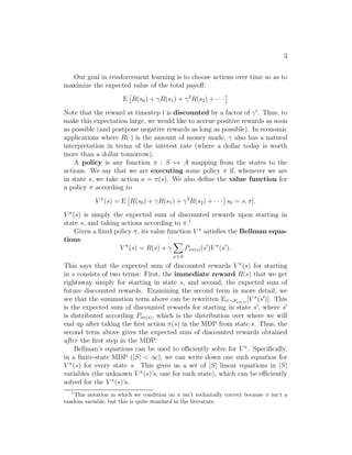
V (s) is simply the expected sum of discounted rewards upon starting in
state s, and taking actions according to π.1
Given a fixed policy π, its value function V satisfies the Bellman equa-
tions:
V (s) = R(s) + γXs′∈S
Ps(s)(s′)V (s′).
This says that the expected sum of discounted rewards V (s) for starting
in s consists of two terms: First, the immediate reward R(s) that we get
rightaway simply for starting in state s, and second, the expected sum of
future discounted rewards. Examining the second term in more detail, we
see that the summation term above can be rewritten Es′∼Ps(s) [V (s′)]. This
is the expected sum of discounted rewards for starting in state s′, where s′
is distributed according Ps(s), which is the distribution over where we will
end up after taking the first action π(s) in the MDP from state s. Thus, the
second term above gives the expected sum of discounted rewards obtained
after the first step in the MDP.
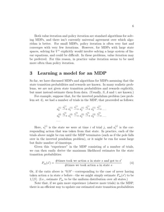
Bellman’s equations can be used to efficiently solve for V . Specifically,
in a finite-state MDP (|S| ∞), we can write down one such equation for
V (s) for every state s. This gives us a set of |S| linear equations in |S|
variables (the unknown V (s)’s, one for each state), which can be efficiently
solved for the V (s)’s.
1This notation in which we condition on isn’t technically correct because isn’t a
random variable, but this is quite standard in the literature.

4
We also define the optimal value function according to
V ∗(s) = max

V (s). (1)
In other words, this is the best possible expected sum of discounted rewards
that can be attained using any policy. There is also a version of Bellman’s
equations for the optimal value function:
V ∗(s) = R(s) + max
a∈A
γXs′∈S
Psa(s′)V ∗(s′). (2)
The first term above is the immediate reward as before. The second term
is the maximum over all actions a of the expected future sum of discounted
rewards we’ll get upon after action a. You should make sure you understand
this equation and see why it makes sense.
We also define a policy π∗ : S7→ A as follows:
a∈A Xs′∈S
π∗(s) = argmax
Psa(s′)V ∗(s′). (3)
Note that π∗(s) gives the action a that attains the maximum in the “max”
in Equation (2).
It is a fact that for every state s and every policy π, we have
V ∗(s) = V ∗
(s) ≥ V (s).
The first equality says that the V ∗ , the value function for π∗, is equal to the
optimal value function V ∗ for every state s. Further, the inequality above
says that π∗’s value is at least a large as the value of any other other policy.
In other words, π∗ as defined in Equation (3) is the optimal policy.
Note that π∗ has the interesting property that it is the optimal policy
for all states s. Specifically, it is not the case that if we were starting in
some state s then there’d be some optimal policy for that state, and if we
were starting in some other state s′ then there’d be some other policy that’s
optimal policy for s′. Specifically, the same policy π∗ attains the maximum
in Equation (1) for all states s. This means that we can use the same policy
π∗ no matter what the initial state of our MDP is.
2 Value iteration and policy iteration
We now describe two efficient algorithms for solving finite-state MDPs. For
now, we will consider only MDPs with finite state and action spaces (|S|
∞, |A| ∞).
The first algorithm, value iteration, is as follows:

5
1. For each state s, initialize V (s) := 0.
2. Repeat until convergence {
For every state, update V (s) := R(s) + maxa∈A γPs′ Psa(s′)V (s′).
}
This algorithm can be thought of as repeatedly trying to update the esti-
mated value function using Bellman Equations (2).
There are two possible ways of performing the updates in the inner loop of
the algorithm. In the first, we can first compute the new values for V (s) for
every state s, and then overwrite all the old values with the new values. This
is called a synchronous update. In this case, the algorithm can be viewed as
implementing a “Bellman backup operator” that takes a current estimate of
the value function, and maps it to a new estimate. (See homework problem
for details.) Alternatively, we can also perform asynchronous updates.
Here, we would loop over the states (in some order), updating the values one
at a time.
Under either synchronous or asynchronous updates, it can be shown that
value iteration will cause V to converge to V ∗. Having found V ∗, we can
then use Equation (3) to find the optimal policy.
Apart from value iteration, there is a second standard algorithm for find-
ing an optimal policy for an MDP. The policy iteration algorithm proceeds
as follows:
1. Initialize π randomly.
2. Repeat until convergence {
(a) Let V := V .
(b) For each state s, let π(s) := argmaxa∈APs′ Psa(s′)V (s′).
}
Thus, the inner-loop repeatedly computes the value function for the current
policy, and then updates the policy using the current value function. (The
policy π found in step (b) is also called the policy that is greedy with re-
spect to V .) Note that step (a) can be done via solving Bellman’s equations
as described earlier, which in the case of a fixed policy, is just a set of |S|
linear equations in |S| variables.
After at most a finite number of iterations of this algorithm, V will con-
verge to V ∗, and π will converge to π∗.

6
Both value iteration and policy iteration are standard algorithms for solv-
ing MDPs, and there isn’t currently universal agreement over which algo-
rithm is better. For small MDPs, policy iteration is often very fast and
converges with very few iterations. However, for MDPs with large state
spaces, solving for V explicitly would involve solving a large system of lin-
ear equations, and could be difficult. In these problems, value iteration may
be preferred. For this reason, in practice value iteration seems to be used
more often than policy iteration.
3 Learning a model for an MDP
So far, we have discussed MDPs and algorithms for MDPs assuming that the
state transition probabilities and rewards are known. In many realistic prob-
lems, we are not given state transition probabilities and rewards explicitly,
but must instead estimate them from data. (Usually, S,A and γ are known.)
For example, suppose that, for the inverted pendulum problem (see prob-
lem set 4), we had a number of trials in the MDP, that proceeded as follows:
s(1)
0
(1)
a
−→ 0 s(1)
1
(1)
a
−→ 1 s(1)
2
(1)
a
−→ 2 s(1)
3
(1)
a
−→ 3 . . .
s(2)
0
(2)
a
−→ 0 s(2)
1
(2)
a
−→ 1 s(2)
2
(2)
a
−→ 2 s(2)
3
(2)
a
−→ 3 . . .
. . .
i is the state we were at time i of trial j, and a(j)
Here, s(j)
i is the cor-
responding action that was taken from that state. In practice, each of the
trials above might be run until the MDP terminates (such as if the pole falls
over in the inverted pendulum problem), or it might be run for some large
but finite number of timesteps.
Given this “experience” in the MDP consisting of a number of trials,
we can then easily derive the maximum likelihood estimates for the state
transition probabilities:
Psa(s′) =
#times took we action a in state s and got to s′
#times we took action a in state s
(4)
Or, if the ratio above is “0/0”—corresponding to the case of never having
taken action a in state s before—the we might simply estimate Psa(s′) to be
1/|S|. (I.e., estimate Psa to be the uniform distribution over all states.)
Note that, if we gain more experience (observe more trials) in the MDP,
there is an efficient way to update our estimated state transition probabilities

7
using the new experience. Specifically, if we keep around the counts for both
the numerator and denominator terms of (4), then as we observe more trials,
we can simply keep accumulating those counts. Computing the ratio of these
counts then given our estimate of Psa.
Using a similar procedure, if R is unknown, we can also pick our estimate
of the expected immediate reward R(s) in state s to be the average reward
observed in state s.
Having learned a model for the MDP, we can then use either value it-
eration or policy iteration to solve the MDP using the estimated transition
probabilities and rewards. For example, putting together model learning and
value iteration, here is one possible algorithm for learning in an MDP with
unknown state transition probabilities:
1. Initialize π randomly.
2. Repeat {
(a) Execute π in the MDP for some number of trials.
(b) Using the accumulated experience in the MDP, update our esti-
mates for Psa (and R, if applicable).
(c) Apply value iteration with the estimated state transition probabil-
ities and rewards to get a new estimated value function V .
(d) Update π to be the greedy policy with respect to V .
}
We note that, for this particular algorithm, there is one simple optimiza-
tion that can make it run much more quickly. Specifically, in the inner loop
of the algorithm where we apply value iteration, if instead of initializing value
iteration with V = 0, we initialize it with the solution found during the pre-
vious iteration of our algorithm, then that will provide value iteration with
a much better initial starting point and make it converge more quickly.
4 Continuous state MDPs
So far, we’ve focused our attention on MDPs with a finite number of states.
We now discuss algorithms for MDPs that may have an infinite number of
states. For example, for a car, we might represent the state as (x, y, θ, ˙ x, ˙ y, ˙θ
),
comprising its position (x, y); orientation θ; velocity in the x and y directions
x˙ and y˙; and angular velocity θ˙. Hence, S = R6 is an infinite set of states,

8
˙ψ
˙because there is an infiθ
˙φ
nite number of possible positions and orientations
for the car.2 Similarly, the inverted pendulum you saw in PS4 has states
(x, θ, x˙ , θ˙), where θ is the angle of the pole. And, a helicopter flying in 3d
space has states of the form (x, y, z, φ, θ, ψ, x, ˙ y, ˙ z, ˙ , , ), where here the roll
φ, pitch θ, and yaw ψ angles specify the 3d orientation of the helicopter.
In this section, we will consider settings where the state space is S = Rn,
and describe ways for solving such MDPs.
4.1 Discretization
Perhaps the simplest way to solve a continuous-state MDP is to discretize
the state space, and then to use an algorithm like value iteration or policy
iteration, as described previously.
For example, if we have 2d states (s1, s2), we can use a grid to discretize
the state space:
Here, each grid cell represents a separate discrete state ¯s. We can then ap-
proximate the continuous-state MDP via a discrete-state one ( ¯ S,A, {P¯sa}, γ,R),
where ¯ S is the set of discrete states, {P¯sa} are our state transition probabil-
ities over the discrete states, and so on. We can then use value iteration or
policy iteration to solve for the V ∗(¯s) and π∗(¯s) in the discrete state MDP
( ¯ S,A, {P¯sa}, γ,R). When our actual system is in some continuous-valued
state s ∈ S and we need to pick an action to execute, we compute the
corresponding discretized state ¯s, and execute action π∗(¯s).
This discretization approach can work well for many problems. However,
there are two downsides. First, it uses a fairly naive representation for V ∗
2Technically, is an orientation and so the range of is better written ∈ [−, ) than
∈ R; but for our purposes, this distinction is not important.

9
(and π∗). Specifically, it assumes that the value function is takes a constant
value over each of the discretization intervals (i.e., that the value function is
piecewise constant in each of the gridcells).
To better understand the limitations of such a representation, consider a
supervised learning problem of fitting a function to this dataset:
1 2 3 4 5 6 7 8
5.5
5
4.5
4
3.5
3
2.5
2
1.5
x
y
Clearly, linear regression would do fine on this problem. However, if we
instead discretize the x-axis, and then use a representation that is piecewise
constant in each of the discretization intervals, then our fit to the data would
look like this:
1 2 3 4 5 6 7 8
5.5
5
4.5
4
3.5
3
2.5
2
1.5
x
y
This piecewise constant representation just isn’t a good representation for
many smooth functions. It results in little smoothing over the inputs, and no
generalization over the different grid cells. Using this sort of representation,
we would also need a very fine discretization (very small grid cells) to get a
good approximation.

10
A second downside of this representation is called the curse of dimen-
sionality. Suppose S = Rn, and we discretize each of the n dimensions of the
state into k values. Then the total number of discrete states we have is kn.
This grows exponentially quickly in the dimension of the state space n, and
thus does not scale well to large problems. For example, with a 10d state, if
we discretize each state variable into 100 values, we would have 10010 = 1020
discrete states, which is far too many to represent even on a modern desktop
computer.
As a rule of thumb, discretization usually works extremely well for 1d
and 2d problems (and has the advantage of being simple and quick to im-
plement). Perhaps with a little bit of cleverness and some care in choosing
the discretization method, it often works well for problems with up to 4d
states. If you’re extremely clever, and somewhat lucky, you may even get it
to work for some 6d problems. But it very rarely works for problems any
higher dimensional than that.
4.2 Value function approximation
We now describe an alternative method for finding policies in continuous-
state MDPs, in which we approximate V ∗ directly, without resorting to dis-
cretization. This approach, caled value function approximation, has been
successfully applied to many RL problems.
4.2.1 Using a model or simulator
To develop a value function approximation algorithm, we will assume that
we have a model, or simulator, for the MDP. Informally, a simulator is
a black-box that takes as input any (continuous-valued) state st and action
at, and outputs a next-state st+1 sampled according to the state transition
probabilities Pstat :
There’re several ways that one can get such a model. One is to use
physics simulation. For example, the simulator for the inverted pendulum

11
in PS4 was obtained by using the laws of physics to calculate what position
and orientation the cart/pole will be in at time t+1, given the current state
at time t and the action a taken, assuming that we know all the parameters
of the system such as the length of the pole, the mass of the pole, and so
on. Alternatively, one can also use an off-the-shelf physics simulation software
package which takes as input a complete physical description of a mechanical
system, the current state st and action at, and computes the state st+1 of the
system a small fraction of a second into the future.3
An alternative way to get a model is to learn one from data collected in
the MDP. For example, suppose we execute m trials in which we repeatedly
take actions in an MDP, each trial for T timesteps. This can be done picking
actions at random, executing some specific policy, or via some other way of
choosing actions. We would then observe m state sequences like the following:
s(1)
0
(1)
a
−→ 0 s(1)
1
(1)
a
−→ 1 s(1)
2
(1)
a
−→ 2 · · ·
(1)
T−1 −→ s(1)
a
T
s(2)
0
(2)
a
−→ 0 s(2)
1
(2)
a
−→ 1 s(2)
2
(2)
a
−→ 2 · · ·
(2)
T−1 −→ s(2)
a
T
· · ·
s(m)
0
(m)
a
0 −→ s(m)
1
(m)
a
1 −→ s(m)
2
(m)
a
2 −→ · · ·
(m)
T−1 −→ s(m)
a
T
We can then apply a learning algorithm to predict st+1 as a function of st
and at.
For example, one may choose to learn a linear model of the form
st+1 = Ast + Bat, (5)
using an algorithm similar to linear regression. Here, the parameters of the
model are the matrices A and B, and we can estimate them using the data
collected from our m trials, by picking
argmin
A,B
m
Xi
=1
T−1
Xt=0

t + Ba(i)
t

s(i)
t+1 − As(i)
2
.
(This corresponds to the maximum likelihood estimate of the parameters.)
Having learned A and B, one option is to build a deterministic model,
in which given an input st and at, the output st+1 is exactly determined.
3Open Dynamics Engine (http://www.ode.com) is one example of a free/open-source
physics simulator that can be used to simulate systems like the inverted pendulum, and
that has been a reasonably popular choice among RL researchers.

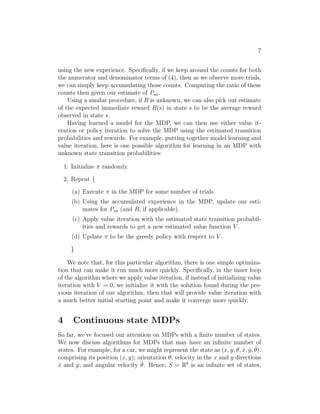
12
Specifically, we always compute st+1 according to Equation (5). Alterna-
tively, we may also build a stochastic model, in which st+1 is a random
function of the inputs, by modelling it as
st+1 = Ast + Bat + ǫt,
where here ǫt is a noise term, usually modeled as ǫt ∼ N(0,). (The covari-
ance matrix can also be estimated from data in a straightforward way.)
Here, we’ve written the next-state st+1 as a linear function of the current
state and action; but of course, non-linear functions are also possible. Specif-
ically, one can learn a model st+1 = Aφs(st) + Bφa(at), where φs and φa are
some non-linear feature mappings of the states and actions. Alternatively,
one can also use non-linear learning algorithms, such as locally weighted lin-
ear regression, to learn to estimate st+1 as a function of st and at. These
approaches can also be used to build either deterministic or stochastic sim-
ulators of an MDP.
4.2.2 Fitted value iteration
We now describe the fitted value iteration algorithm for approximating
the value function of a continuous state MDP. In the sequel, we will assume
that the problem has a continuous state space S = Rn, but that the action
space A is small and discrete.4
Recall that in value iteration, we would like to perform the update
a Zs′
V (s) := R(s) + γ max
Psa(s′)V (s′)ds′ (6)
= R(s) + γ max
a
Es′∼Psa [V (s′)] (7)
(In Section 2, we had written the value iteration update with a summation
V (s) := R(s) + γ maxaPs′ Psa(s′)V (s′) rather than an integral over states;
the new notation reflects that we are now working in continuous states rather
than discrete states.)
The main idea of fitted value iteration is that we are going to approxi-
mately carry out this step, over a finite sample of states s(1), . . . , s(m). Specif-
ically, we will use a supervised learning algorithm—linear regression in our
4In practice, most MDPs have much smaller action spaces than state spaces. E.g., a car
has a 6d state space, and a 2d action space (steering and velocity controls); the inverted
pendulum has a 4d state space, and a 1d action space; a helicopter has a 12d state space,
and a 4d action space. So, discretizing ths set of actions is usually less of a problem than
discretizing the state space would have been.

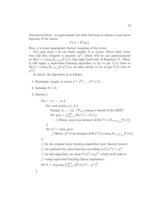
13
description below—to approximate the value function as a linear or non-linear
function of the states:
V (s) = θTφ(s).
Here, φ is some appropriate feature mapping of the states.
For each state s in our finite sample of m states, fitted value itera-
tion will first compute a quantity y(i), which will be our approximation
to R(s) + γ maxa Es′∼Psa[V (s′)] (the right hand side of Equation 7). Then,
it will apply a supervised learning algorithm to try to get V (s) close to
R(s) + γ maxa Es′∼Psa [V (s′)] (or, in other words, to try to get V (s) close to
y(i)).
In detail, the algorithm is as follows:
1. Randomly sample m states s(1), s(2), . . . s(m) ∈ S.
2. Initialize θ := 0.
3. Repeat {
For i = 1, . . . ,m {
For each action a ∈ A {
Sample s′
k ∼ Ps(i)a (using a model of the MDP).
1, . . . , s′
k Pk
Set q(a) = 1
j=1 R(s(i)) + γV (s′
j)
// Hence, q(a) is an estimate of R(s(i))+γEs′∼P
s(i)a
[V (s′)].
}
Set y(i) = maxa q(a).
// Hence, y(i) is an estimate of R(s(i))+γ maxa Es′∼P
s(i)a
[V (s′)].
}
// In the original value iteration algorithm (over discrete states)
// we updated the value function according to V (s(i)) := y(i).
// In this algorithm, we want V (s(i)) ≈ y(i), which we’ll achieve
// using supervised learning (linear regression).
Set θ := argmin
i=1 θTφ(s(i)) − y(i)2
1
2 Pm
}

Machine learning (13)

Recommended

Recommended

More Related Content

What's hot

What's hot (18)

Viewers also liked

Viewers also liked (11)

Similar to Machine learning (13)

Similar to Machine learning (13) (20)

More from NYversity

More from NYversity (20)

Recently uploaded

Recently uploaded (20)

Machine learning (13)