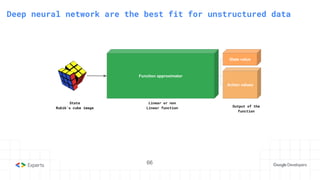
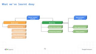
Azzeddine CHENINE
Research Engineer, Applied RL @InstaDeep | ML GDE
@azzeddineCH_
Head First
Reinforcement Learning
Hi
I am a Research Engineer in Applied RL
at InstaDeep and ML GDE
For the past the 3 years, I worked on
applying scalable DeepRL methods
application for placement on system
on chips and routing for printed circuit
boards
Reinforcement Learning
An introduction
AI and Reinforcement
Learning
Machine Learning
The science of getting computers to act without being explicitly
programmed.
- Andrew Ng -
5
6
Classify physical activity using explicit rules
7
Classify physical activity using learnable rules
󰪦
Why these models are labeled as smart
Machine Learning models are able to learn to make decisions to
achieve a predetermined goal
8
9
Key types of Machine Learning tasks
Supervised
Learning
Unsupervised
Learning
Clustering
Association
Regression
Classification Translation
Identify population groups
Recommending products Recommending friends
Weather forecasting
Object
detection
Generate Image based
on latent Variables
10
All tasks optimize a prediction loss
- Mean squared error loss
- Cross entropy loss
- Categorical cross entropy loss
- Cosine similarity loss
And many more ...
Using Stochastic gradient descent Algorithm
to optimize an objective function:
Tasks optimize for a goal by taking a
sequence of decision within an
environment
11
12
Sequential decision making tasks
Winning a chess game Driving a car home Scoring a goal
13
Sequential decision making via Reinforcement Learning
Winning a chess game
- Optimise behavior based on a feedback signal (Reward)
- Learn an optimal behavior (policy) by interactions
with the world (environment) without provided examples
by interacting
- The feedback signal (Reward) on your actions can be
immediate or deferred (win or lose the game)
- The quality of the action you take depends on the current
state and the final outcome of the task (episode)
Definitions
15
1. The Reinforcement Learning framework
Environment
Agent
Reward
Next
observation
Action
- The agent interacts with an environment
within a finite horizon (episode)
- At each step t:
- Environment emits observation Oₜ
- Agent chooses an action Aₜ
- Environment executes the agent action
- Environment emits the reward Rₜ₊₁ and next observation Oₜ₊₁
The reward hypothesis
Any goal can be formalized as the outcome of maximizing a
cumulative reward
16
17
2. The Rewards hypothesis
- A reward Rₜ indicates how well the agent is doing at timestep t
- The goal is to maximize the cumulative reward for the given task collected within an episode
- The episode return of state Sₜ depends on the sequence of actions that follows.
- The return can be discounted by 0 ≤ 𝛄 ≤ 1 to determine how much the agents cares about rewards in
the distant future relative to those in the immediate future.
For the rest of the presentation 𝛄 = 1
Estimators in maths
Estimation means having a rough calculation of the value, number,
quantity, or extent of something
18
19
3. State Value function V(s)
- V(Sₜ) represents the expected return (cumulative reward) starting from state Sₜ and picking
actions following a policy
- Since we can define the return recursively 󰗉
20
3. State-Action Value function
4. State-Action Value function q(s,a)
- q(sₜ, a) represents the expected return (cumulative reward) starting from state sₜ and taking
action a then continue picking actions following a policy
- Given state action value function, we can derive a policy by picking the action corresponding to
highest Q value (Q-learning https://arxiv.org/abs/1312.5602)
20
21
3. State-Action Value function
5. Agent observation
- The agent observation is a mapped from the environment state, Oₜ = f(Sₜ).
- The agent observation is not necessarily equal to the environment state.
- The environment is fully observable if Oₜ = Sₜ
- The environment is partially observable if Oₜʹ = Oₜ and Sₜʹ = Sₜ
21
Partially observed
environemnt
22
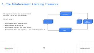
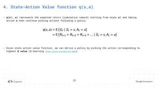
- A mathematical formulation of the agent interaction with the environment
- It requires that the environment is fully observable
6. Markov decision process
- An MDP is a tuple (S, A, p, γ) where:
- S is the set of all possible states
- A is the set of all possible actions
- p(r,s′ | s,a) is the transition function or joint probability of a reward r and next state s′,
given a state s and action a
- γ ∈ [0, 1] is a discount factor that trades off later rewards to earlier ones
Markov decision principal
The Future is independent from the past given the present
The current state summarizes the history of the agent
23
24
- Given the full horizon
Hₜ
7. Markovian state
- A state is called markovian only if
- If the environment is partially observable then the state is not Markovian
- We can turn a state to a Markovian state by stacking horizon data
Markovian state
Non Markovian state
Recap
- MDP is the representation of the agent-environment interaction
25
- Every RL problem can be formulated to a reward goal
- Agent components are: State, Value function, Policy, the world model
Check your understanding
Fill in the value of each state
26
27
3. State-Action Value function
- Actions: N, E, S, W
- Reward: -1 for each step
27
28
3. State-Action Value function
- Actions: N, E, S, W
- Reward: -1 for each step
Optimal policy
28
29
3. State-Action Value function
- Actions: N, E, S, W
- Reward: -1 for each step
Optimal policy State value function
29
RL subproblems
31
3. State-Action Value function
1. Prediction and Control
- Prediction: given a policy, we can predict (evaluate) the future return given the current state
(learn value function)
- Control: improve your actions choices (learn policy function)
- Prediction and control can be strongly related
31
32
3. State-Action Value function
2. Learning and Planning
- At first, the environment can be unknown to the agent.
- The agent learn the model of the world by interaction and exploration
- Once the model is learnt (sometime given ie: chess), the agent start planning actions to reach
optimal policy
32
Solving RL
Prediction,control problems
Tabular solution
method
35
3. State-Action Value function
Tabular MDPs explained
- The state and action space is small enough to be represented by arrays or tables
- Given the exact quantification of the possible states and actions, we can find exactly the optimal
solution for the prediction (value function) and control (policy) problems
- 27 states
- 4 actions
- A reward of -1 for each step
35
Dynamic Programming
Definition
The term dynamic programming (DP) refers to a collection of
algorithms that can be used to compute optimal policies given a
perfect model of the environment as a Markov decision process (MDP).
- Richard S.Sutton and Andrew G. Barto -
37
38
3. State-Action Value function
1. Policy Evaluation
- Given an arbitrary policy π ,we want to compute the corresponding state value function V𝜋
- We iteratively iterate over all the states and update the state value using the equation
below until we reach a state of convergence
38
39
3. State-Action Value function
1. Policy Evaluation
39
40
3. State-Action Value function
2. Policy Improvement
- The goal of computing the value function for a policy is to help find a better policy
- Given the new value function, we can define the new policy
40
41
3. State-Action Value function
3. Policy Iteration
41
42
3. State-Action Value function
3. Recap
42
Monte Carlo methods
Notes
Monte Carlo methods require only experience—sample sequences of
states, actions, and rewards from actual or simulated interaction
with an environment without the need for the full probability
distribution of state, reward over actions
- Richard S.Sutton and Andrew G. Barto -
44
45
3. State-Action Value function
1. First visit Monte-Carlo for prediction
- Given an arbitrary policy π ,we can estimate V𝜋
- Once the Algorithm converges we can move to policy improvement
- An acceptable estimate of Gₜ would be the average of all the encountered discounted
returns after infinite visits to the state Gₜ
45
46
3. State-Action Value function
1. First visit Monte-Carlo for prediction
46
47
3. State-Action Value function
2. First visit Monte-Carlo for control
- Given an arbitrary initial policy π ,we can estimate state action value V𝜋.
- Instead of averaging the return of the visited state Sₜ, we average the return of the
visited state action pair Sₜ, Aₜ .
- The new policy can be calculated by choosing the action corresponding to best Q value
47
48
3. State-Action Value function
2. First visit Monte-Carlo for control
48
Exploration vs Exploitation problem
49
All learning control methods face a dilemma: they seek to learn
action values conditional on subsequent optimal behavior, but they
need to behave non-optimally in order to explore all actions
- Richard S.Sutton and Andrew G. Barto -
50
3. State-Action Value function
Off policy and On policy methods
- Learning control methods fall into two categories: off policy and on policy methods
- On policy methods update the current policy using the data generated by the former (which
what we have been doing so far)
- Off policy methods update the current policy using data generated by two policies
- Target policy: the current policy being learned about
- Behavior policy: the policy responsible of generating a exploratory behavior ( random
actions, data generated by old policies )
50
51
3. State-Action Value function
3. Monte-Carlo Generalized Policy Iteration
- Sample episode 1, . . ., k, . . ., using π: {S₁, A₂, R₂, ..., Sₜ } ∼ π
- For each state St and action At in the episode
- Improve policy based on new action-value function
51
Problems with MC methods
- High variance given
52
- Waiting until the end of the of the episode
Temporal Difference
Learning 💰
54
3. State-Action Value function
TD-learning explained
- TD-learning is a combination of monte-carlo and dynamic programming ideas.
- It is the backbone of most of state of the art Deep Reinforcement Learning algorithm DQN, PPO ...
- Like DP, TD-learning update the estimate based on another estimate. We call this Bootstrapping
- Like MC, TD-L learns directly from experiences without the need for a model of the environment.
54
55
3. State-Action Value function
1. TD Prediction
- MC methods uses the episode return Gₜ as the target for the value for Sₜ.
- Unlike MC methods, TD methods update the value at each step and use an estimate of
Gₜ, we call the TD-Target.
55
56
3. State-Action Value function
1. TD-Learning for prediction
56
57
3. State-Action Value function
1. Example of MC vs TD prediction
- we are driving home from work and we try
to estimate how long it will take us.
- At each step, we re-estimated our time
because of complications (e.g. car
doesn’t work, highway is busy, etc).
- How can we update our estimate of the
time it takes to get home for next time
we leave work?
57
58
3. State-Action Value function
1. Example of MC vs TD prediction
- we are driving home from work and we try
to estimate how long it will take us.
- At each step, we re-estimated our time
because of complications (e.g. car
doesn’t work, highway is busy, etc).
- How can we update our estimate of the
time it takes to get home for next time
we leave work?
Monte Carlo TD-Learning
58
59
3. State-Action Value function
2. Sarsa: On Policy TD Control
- Similarly to MC method, we learn a policy by learning the action value function Q(S,A)
- The Algorithm is called Sarsa as it relies on transition { state, action, reward }
- Theis Algorithm is the backbone to the famous Deep Q-learning paper
59
60
3. State-Action Value function
2. Sarsa: On Policy TD Control
60
61
3. State-Action Value function
3. Q-learning (max sarsa): Off Policy TD Control
61
Recap of Tabular
solution methods
63
3. State-Action Value function
Dynamic programming
Policy Evaluation
Policy Improvement
Value Iteration
Tabular solution methods
Model based Model free
Monte Carlo methods
TD-learning methods
1. The family of tabular solution methods
63
Approximate solution
methods
OpenAI: solving the rubix cube using a single handed robot
- The robots observes the world
through camera lenses,
censors..ect
- The state space is infinite and
it's not practical to store in
a table
- The state space consists of a
set of unstructured data and
not tabular data
65
Deep neural network are the best fit for unstructured data
Function approximator
Action values
State value
State
Rubik's cube image
Linear or non
Linear function Output of the
function
66
Gradient based
methods
Function derivatives and Gradient
68
- The derivative of a function f measure the sensitivity to change
with respect to the argument x
- The gradient of a function with respect to x, measure by how much x
needs to change so we reach a minimum
Function derivative and gradient
Gradient -4 Gradient -1 Gradient 0
69
70
1. Value function approximation
- Given a function approximator with a set of
weights 𝔀, minimize 𝘑(w)
- Using stochastic Gradient Descent
algorithms we form a good estimator for the
loss
- The loss target can be the MC return of the
TD target.
2. Policy function approximation (home work 😄)
71
72
3. State-Action Value function
Dynamic programming
Policy Evaluation
Policy Improvement
Value Iteration
Tabular solution
methods
Model based Model free
Monte Carlo methods
TD-learning methods
What we've learnt doay
Value approximation
Approximation
method
Policy gradient
72
References
Reinforcement Learning
An introduction
Deep Reinforcement Learning
Lectures from DeepMind 2021
Questions ?

Head First Reinforcement Learning

  • 1.
    Azzeddine CHENINE Research Engineer,Applied RL @InstaDeep | ML GDE @azzeddineCH_ Head First Reinforcement Learning
  • 2.
    Hi I am aResearch Engineer in Applied RL at InstaDeep and ML GDE For the past the 3 years, I worked on applying scalable DeepRL methods application for placement on system on chips and routing for printed circuit boards
  • 3.
  • 4.
  • 5.
    Machine Learning The scienceof getting computers to act without being explicitly programmed. - Andrew Ng - 5
  • 6.
    6 Classify physical activityusing explicit rules
  • 7.
    7 Classify physical activityusing learnable rules 󰪦
  • 8.
    Why these modelsare labeled as smart Machine Learning models are able to learn to make decisions to achieve a predetermined goal 8
  • 9.
    9 Key types ofMachine Learning tasks Supervised Learning Unsupervised Learning Clustering Association Regression Classification Translation Identify population groups Recommending products Recommending friends Weather forecasting Object detection Generate Image based on latent Variables
  • 10.
    10 All tasks optimizea prediction loss - Mean squared error loss - Cross entropy loss - Categorical cross entropy loss - Cosine similarity loss And many more ... Using Stochastic gradient descent Algorithm to optimize an objective function:
  • 11.
    Tasks optimize fora goal by taking a sequence of decision within an environment 11
  • 12.
    12 Sequential decision makingtasks Winning a chess game Driving a car home Scoring a goal
  • 13.
    13 Sequential decision makingvia Reinforcement Learning Winning a chess game - Optimise behavior based on a feedback signal (Reward) - Learn an optimal behavior (policy) by interactions with the world (environment) without provided examples by interacting - The feedback signal (Reward) on your actions can be immediate or deferred (win or lose the game) - The quality of the action you take depends on the current state and the final outcome of the task (episode)
  • 14.
  • 15.
    15 1. The ReinforcementLearning framework Environment Agent Reward Next observation Action - The agent interacts with an environment within a finite horizon (episode) - At each step t: - Environment emits observation Oₜ - Agent chooses an action Aₜ - Environment executes the agent action - Environment emits the reward Rₜ₊₁ and next observation Oₜ₊₁
  • 16.
    The reward hypothesis Anygoal can be formalized as the outcome of maximizing a cumulative reward 16
  • 17.
    17 2. The Rewardshypothesis - A reward Rₜ indicates how well the agent is doing at timestep t - The goal is to maximize the cumulative reward for the given task collected within an episode - The episode return of state Sₜ depends on the sequence of actions that follows. - The return can be discounted by 0 ≤ 𝛄 ≤ 1 to determine how much the agents cares about rewards in the distant future relative to those in the immediate future. For the rest of the presentation 𝛄 = 1
  • 18.
    Estimators in maths Estimationmeans having a rough calculation of the value, number, quantity, or extent of something 18
  • 19.
    19 3. State Valuefunction V(s) - V(Sₜ) represents the expected return (cumulative reward) starting from state Sₜ and picking actions following a policy - Since we can define the return recursively 󰗉
  • 20.
    20 3. State-Action Valuefunction 4. State-Action Value function q(s,a) - q(sₜ, a) represents the expected return (cumulative reward) starting from state sₜ and taking action a then continue picking actions following a policy - Given state action value function, we can derive a policy by picking the action corresponding to highest Q value (Q-learning https://arxiv.org/abs/1312.5602) 20
  • 21.
    21 3. State-Action Valuefunction 5. Agent observation - The agent observation is a mapped from the environment state, Oₜ = f(Sₜ). - The agent observation is not necessarily equal to the environment state. - The environment is fully observable if Oₜ = Sₜ - The environment is partially observable if Oₜʹ = Oₜ and Sₜʹ = Sₜ 21 Partially observed environemnt
  • 22.
    22 - A mathematicalformulation of the agent interaction with the environment - It requires that the environment is fully observable 6. Markov decision process - An MDP is a tuple (S, A, p, γ) where: - S is the set of all possible states - A is the set of all possible actions - p(r,s′ | s,a) is the transition function or joint probability of a reward r and next state s′, given a state s and action a - γ ∈ [0, 1] is a discount factor that trades off later rewards to earlier ones
  • 23.
    Markov decision principal TheFuture is independent from the past given the present The current state summarizes the history of the agent 23
  • 24.
    24 - Given thefull horizon Hₜ 7. Markovian state - A state is called markovian only if - If the environment is partially observable then the state is not Markovian - We can turn a state to a Markovian state by stacking horizon data Markovian state Non Markovian state
  • 25.
    Recap - MDP isthe representation of the agent-environment interaction 25 - Every RL problem can be formulated to a reward goal - Agent components are: State, Value function, Policy, the world model
  • 26.
    Check your understanding Fillin the value of each state 26
  • 27.
    27 3. State-Action Valuefunction - Actions: N, E, S, W - Reward: -1 for each step 27
  • 28.
    28 3. State-Action Valuefunction - Actions: N, E, S, W - Reward: -1 for each step Optimal policy 28
  • 29.
    29 3. State-Action Valuefunction - Actions: N, E, S, W - Reward: -1 for each step Optimal policy State value function 29
  • 30.
  • 31.
    31 3. State-Action Valuefunction 1. Prediction and Control - Prediction: given a policy, we can predict (evaluate) the future return given the current state (learn value function) - Control: improve your actions choices (learn policy function) - Prediction and control can be strongly related 31
  • 32.
    32 3. State-Action Valuefunction 2. Learning and Planning - At first, the environment can be unknown to the agent. - The agent learn the model of the world by interaction and exploration - Once the model is learnt (sometime given ie: chess), the agent start planning actions to reach optimal policy 32
  • 33.
  • 34.
  • 35.
    35 3. State-Action Valuefunction Tabular MDPs explained - The state and action space is small enough to be represented by arrays or tables - Given the exact quantification of the possible states and actions, we can find exactly the optimal solution for the prediction (value function) and control (policy) problems - 27 states - 4 actions - A reward of -1 for each step 35
  • 36.
  • 37.
    Definition The term dynamicprogramming (DP) refers to a collection of algorithms that can be used to compute optimal policies given a perfect model of the environment as a Markov decision process (MDP). - Richard S.Sutton and Andrew G. Barto - 37
  • 38.
    38 3. State-Action Valuefunction 1. Policy Evaluation - Given an arbitrary policy π ,we want to compute the corresponding state value function V𝜋 - We iteratively iterate over all the states and update the state value using the equation below until we reach a state of convergence 38
  • 39.
    39 3. State-Action Valuefunction 1. Policy Evaluation 39
  • 40.
    40 3. State-Action Valuefunction 2. Policy Improvement - The goal of computing the value function for a policy is to help find a better policy - Given the new value function, we can define the new policy 40
  • 41.
    41 3. State-Action Valuefunction 3. Policy Iteration 41
  • 42.
    42 3. State-Action Valuefunction 3. Recap 42
  • 43.
  • 44.
    Notes Monte Carlo methodsrequire only experience—sample sequences of states, actions, and rewards from actual or simulated interaction with an environment without the need for the full probability distribution of state, reward over actions - Richard S.Sutton and Andrew G. Barto - 44
  • 45.
    45 3. State-Action Valuefunction 1. First visit Monte-Carlo for prediction - Given an arbitrary policy π ,we can estimate V𝜋 - Once the Algorithm converges we can move to policy improvement - An acceptable estimate of Gₜ would be the average of all the encountered discounted returns after infinite visits to the state Gₜ 45
  • 46.
    46 3. State-Action Valuefunction 1. First visit Monte-Carlo for prediction 46
  • 47.
    47 3. State-Action Valuefunction 2. First visit Monte-Carlo for control - Given an arbitrary initial policy π ,we can estimate state action value V𝜋. - Instead of averaging the return of the visited state Sₜ, we average the return of the visited state action pair Sₜ, Aₜ . - The new policy can be calculated by choosing the action corresponding to best Q value 47
  • 48.
    48 3. State-Action Valuefunction 2. First visit Monte-Carlo for control 48
  • 49.
    Exploration vs Exploitationproblem 49 All learning control methods face a dilemma: they seek to learn action values conditional on subsequent optimal behavior, but they need to behave non-optimally in order to explore all actions - Richard S.Sutton and Andrew G. Barto -
  • 50.
    50 3. State-Action Valuefunction Off policy and On policy methods - Learning control methods fall into two categories: off policy and on policy methods - On policy methods update the current policy using the data generated by the former (which what we have been doing so far) - Off policy methods update the current policy using data generated by two policies - Target policy: the current policy being learned about - Behavior policy: the policy responsible of generating a exploratory behavior ( random actions, data generated by old policies ) 50
  • 51.
    51 3. State-Action Valuefunction 3. Monte-Carlo Generalized Policy Iteration - Sample episode 1, . . ., k, . . ., using π: {S₁, A₂, R₂, ..., Sₜ } ∼ π - For each state St and action At in the episode - Improve policy based on new action-value function 51
  • 52.
    Problems with MCmethods - High variance given 52 - Waiting until the end of the of the episode
  • 53.
  • 54.
    54 3. State-Action Valuefunction TD-learning explained - TD-learning is a combination of monte-carlo and dynamic programming ideas. - It is the backbone of most of state of the art Deep Reinforcement Learning algorithm DQN, PPO ... - Like DP, TD-learning update the estimate based on another estimate. We call this Bootstrapping - Like MC, TD-L learns directly from experiences without the need for a model of the environment. 54
  • 55.
    55 3. State-Action Valuefunction 1. TD Prediction - MC methods uses the episode return Gₜ as the target for the value for Sₜ. - Unlike MC methods, TD methods update the value at each step and use an estimate of Gₜ, we call the TD-Target. 55
  • 56.
    56 3. State-Action Valuefunction 1. TD-Learning for prediction 56
  • 57.
    57 3. State-Action Valuefunction 1. Example of MC vs TD prediction - we are driving home from work and we try to estimate how long it will take us. - At each step, we re-estimated our time because of complications (e.g. car doesn’t work, highway is busy, etc). - How can we update our estimate of the time it takes to get home for next time we leave work? 57
  • 58.
    58 3. State-Action Valuefunction 1. Example of MC vs TD prediction - we are driving home from work and we try to estimate how long it will take us. - At each step, we re-estimated our time because of complications (e.g. car doesn’t work, highway is busy, etc). - How can we update our estimate of the time it takes to get home for next time we leave work? Monte Carlo TD-Learning 58
  • 59.
    59 3. State-Action Valuefunction 2. Sarsa: On Policy TD Control - Similarly to MC method, we learn a policy by learning the action value function Q(S,A) - The Algorithm is called Sarsa as it relies on transition { state, action, reward } - Theis Algorithm is the backbone to the famous Deep Q-learning paper 59
  • 60.
    60 3. State-Action Valuefunction 2. Sarsa: On Policy TD Control 60
  • 61.
    61 3. State-Action Valuefunction 3. Q-learning (max sarsa): Off Policy TD Control 61
  • 62.
  • 63.
    63 3. State-Action Valuefunction Dynamic programming Policy Evaluation Policy Improvement Value Iteration Tabular solution methods Model based Model free Monte Carlo methods TD-learning methods 1. The family of tabular solution methods 63
  • 64.
  • 65.
    OpenAI: solving therubix cube using a single handed robot - The robots observes the world through camera lenses, censors..ect - The state space is infinite and it's not practical to store in a table - The state space consists of a set of unstructured data and not tabular data 65
  • 66.
    Deep neural networkare the best fit for unstructured data Function approximator Action values State value State Rubik's cube image Linear or non Linear function Output of the function 66
  • 67.
  • 68.
    Function derivatives andGradient 68 - The derivative of a function f measure the sensitivity to change with respect to the argument x - The gradient of a function with respect to x, measure by how much x needs to change so we reach a minimum
  • 69.
    Function derivative andgradient Gradient -4 Gradient -1 Gradient 0 69
  • 70.
    70 1. Value functionapproximation - Given a function approximator with a set of weights 𝔀, minimize 𝘑(w) - Using stochastic Gradient Descent algorithms we form a good estimator for the loss - The loss target can be the MC return of the TD target.
  • 71.
    2. Policy functionapproximation (home work 😄) 71
  • 72.
    72 3. State-Action Valuefunction Dynamic programming Policy Evaluation Policy Improvement Value Iteration Tabular solution methods Model based Model free Monte Carlo methods TD-learning methods What we've learnt doay Value approximation Approximation method Policy gradient 72
  • 73.
  • 74.
  • 75.
  • 76.