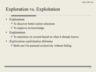
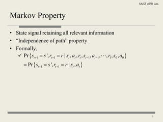
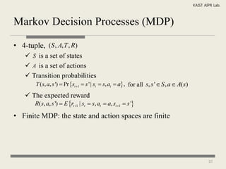
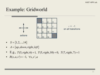
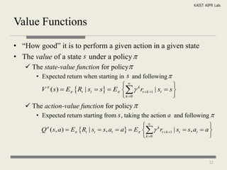
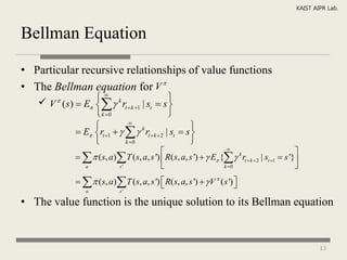
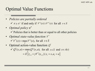
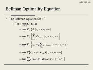
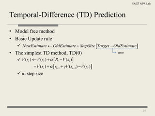
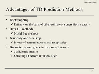
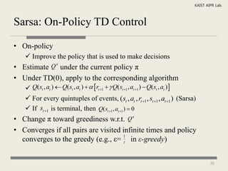
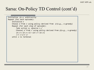
Reinforcement Learning: An Introduction
               Ch. 3, 4, 6
         R. Sutton and A. Barto.


            KAIST AIPR Lab.
             Jung-Yeol Lee
              3rd June 2010


                                          1
KAIST AIPR Lab.


Contents

•   Reinforcement learning
•   Markov decision processes
•   Value function
•   Policy iteration
•   Value iteration
•   Sarsa
•   Q-learning


                                         2
KAIST AIPR Lab.


Reinforcement Learning

• An approach to machine learning
• How to take actions in an environment responding to those
  actions and presenting new situations
• To find a policy that maps situations to the actions
• To discover which action yield the most reward signal over the
  long run


                                                                   3
KAIST AIPR Lab.


Agent-Environment Interface

• Agent
    The learner and decision maker
• Environment
    Everything outside the agent
    Responding to actions and presenting new situations
    Giving a reward (feedback, or reinforcement)


                                                                    4
KAIST AIPR Lab.


Agent-Environment Interface (cont’d)
                       state st
                                           Agent
                              reward r t                action at

                                  st+1
                                          Environment
                                  r t+1

• Agent and environment interact at time steps t  0,1, 2,3,...
    The environment’s state, st  S where S is the set of possible states
    An action, at  A(st ) where A( st ) is the set of actions available in
     state st
    A numerical reward, rt 1 
• Agent’s policy,  t
     t ( s, a), the probability that at  a if st  s
     t (s)  A(s), the deterministic policy

                                                                                 5
KAIST AIPR Lab.


Goals and Rewards

• Goal
   What we want to achieve, not how we want to achieve it
• Rewards
   To formalize the idea of a goal
   A numerical value by the environment.


                                                                      6
KAIST AIPR Lab.


Returns

• Specific function of the reward sequence
• Types of returns
    Episodic tasks
       Rt  rt 1  rt 2  rt 3     rT , where T is a final time step
    Continuing tasks ( T   )
       The additional concept, discount rate        
                                              
       Rt  rt 1   rt  2   rt 3 
                                2
                                              k rt  k 1 , where 0    1
                                             k 0


                                                                                     7
KAIST AIPR Lab.


Exploration vs. Exploitation

• Exploration
    To discover better action selections
    To improve its knowledge
• Exploitation
    To maximize its reward based on what it already knows
• Exploration-exploitation dilemma
    Both can’t be pursued exclusively without failing


                                                                      8
KAIST AIPR Lab.


Markov Property

• State signal retaining all relevant information
• “Independence of path” property
• Formally,
    Pr st 1  s ', rt 1  r | st , at , rt , st 1 , at 1 , , r1 , s0 , a0 
          Pr st 1  s ', rt 1  r | st , at 


                                                                                             9
KAIST AIPR Lab.


Markov Decision Processes (MDP)

• 4-tuple, (S , A, T , R)
     S is a set of states
     A is a set of actions
     Transition probabilities
        T (s, a, s ')  Pr st 1  s ' | st  s, at  a , for all s, s '  S , a  A(s)
     The expected reward
        R(s, a, s ')  E rt 1 | st  s, at  a, st 1  s '

• Finite MDP: the state and action spaces are finite


                                                                                                    10
KAIST AIPR Lab.


Example: Gridworld


•   S  1, 2,...,14
•   A  up, down, right , left
•   E.g., T (5, right ,6)  1, T (5, right ,10)  0, T (7, right ,7)  1
•   R(s, a, s ')  1, s, s ', a


                                                                                   11
KAIST AIPR Lab.


Value Functions

• “How good” it is to perform a given action in a given state
• The value of a state s under a policy 
    The state-value function for policy
      • Expected return when starting in s and following 
                                        k                    
        V ( s)  E Rt | st  s  E   rt  k 1 | st  s 
          

                                        k 0                  
    The action-value function for policy 
      • Expected return starting from s , taking the action a and following 
                                                    k                            
         Q ( s, a)  E Rt | st  s, at  a  E   rt  k 1 | st  s, at  a 
           

                                                    k 0                          


                                                                                   12
KAIST AIPR Lab.


Bellman Equation

• Particular recursive relationships of value functions
• The Bellman equation for V 
    V ( s)  E   rt  k 1 | st  s 
                 k
                                              
                  k 0                       
                            
                                                      
             E rt 1     k rt  k  2 | st  s 
                           k 0                      
                                                                     
                                                                                                    
                  ( s, a) T ( s, a, s ')  R( s, a, s ')   E {  k rt  k  2 | st 1  s '}
                 a          s'                                      k 0                           
                  ( s, a) T ( s, a, s ')  R( s, a, s ')   V  ( s ') 
                                                                           
                  a             s'

• The value function is the unique solution to its Bellman equation


                                                                                                            13
KAIST AIPR Lab.


Optimal Value Functions

• Policies are partially ordered
       ' if and only if V  (s)  V  ' (s) for all s  S
• Optimal policy π*
     Policies that is better than or equal to all other policies
• Optimal state-value function V *
    V * (s)  max V  ( s), for all s  S
                
• Optimal action-value function Q*
     Q* (s, a)  max Q ( s, a), for all s  S and a  A(s)
                   
                 E rt 1   V * (st 1 ) | st  s, at  a


                                                                            14
KAIST AIPR Lab.


Bellman Optimality Equation

• The Bellman equation for V *
                             *
     V ( s)  max Q ( s, a)
      *
             aA( s )

            max E * Rt | st  s, at  a
                a

                       k                                
            max E *   rt  k 1 | st  s, at  a 
              a
                       k 0                              
                                 
                                                                   
            max E * rt 1     k rt  k  2 | st  s, at  a 
              a
                                k 0                              
            max E rt 1   V * (st 1 ) | st  s, at  a
                a


            max  T ( s, a, s ')  R( s, a, s ')   V * ( s ') 
                                                                
                a
                        s'


                                                                               15
KAIST AIPR Lab.


Bellman Optimality Equation (cont’d)

• The Bellman optimality equation for Q*
                      
    Q* (s, a)  E rt 1   max Q* (st 1 , a ') | st  s, at  a
                              a'
                                                                        
                   T (s, a, s ')  R( s, a, s ')   max Q* ( s ', a ') 
                   s'
                                                       a'                

• Optimal policy from Q*
     * (s)  arg max Q* (s, a)
                  aA( s )

• Optimal policy from V *
    Any policy that is greedy with respect to V * (s)  max Q (s, a)
                                                                                         *


                                                                              aA( s )


                                                                                                     16
KAIST AIPR Lab.


Dynamic Programming (DP)

• Algorithms for optimal policies under a perfect model
• Limited utility in reinforcement learning, but theoretically
  important
• Foundation for the understanding of other methods


                                                                    17
KAIST AIPR Lab.


Policy Evaluation

• How to compute the state-value function V 
• Recall, the Bellman equation for V 
    V (s)    ( s, a) T ( s, a, s ')  R( s, a, s ')   V ( s ') 
                                                             
                                                                     
                  a           s'

• A sequence of approximate value functions V0 ,V1 ,V2 ,
• Successive approximation
    Vk 1 ( s)   T ( s, a, s ')  R( s, a, s ')   Vk ( s ') 
                       s'
• Vk converge to V  as k  


                                                                                  18
KAIST AIPR Lab.


Policy Improvement

• Policy improvement theorem (proof)
     If Q (s,  '(s))  V  (s), for all s  S then, V  ' (s)  V  (s)
     Better to switch action iff Q (s,  '(s))  V  (s)
• The new greedy policy,  '
     Selecting the action that appears best
        '(s)  arg max Q ( s, a)
                       a

               arg max  T ( s, a, s ')  R( s, a, s ')   V  ( s ') 
                                                                       
                       a
                            s'


• What if V  '  V  ?
     Both     ' and           are optimal policies


                                                                                     19
KAIST AIPR Lab.


Policy Iteration

•  0  V   1  V    2    *  V * ,
       E
          0    I
                       E1
                              I
                                      E
                                              I
                                                   E
                                                      
  where  denotes a policy evaluation and
            E
              
            denotes a policy improvement
            I
              
• Policy iteration finishes when a policy is stable


                                                              20
KAIST AIPR Lab.


Policy Iteration (cont’d)
 Initialization
 V (s)  and arbitrarily for all

 Policy Evaluation
 repeat
       0
       for each s  S do
               v  V (s)
               V (s)   s ' T (s,  (s), s ')  R(s,  ( s), s ')   V ( s ') 
                 max(, v  V (s) )
     end for
 until    (a small positive number)

 Policy Improvement
 policy  stable  true
 for all s  S do
       b   ( s)
        (s)  arg max a  s ' T (s, a, s ')  R(s, a, s ')   V (s ')
     If b   (s) then policy  stable  false
 end for
 If policy  stable then stop; else go to Policy evaluation


                                                                                            21
KAIST AIPR Lab.


Value Iteration

• Turning the Bellman optimality equation into an update rule
    Vk 1 (s)  max E rt 1   Vk (st 1 ) | st  s, at  a
                         a

                      max  T ( s, a, s ')  R(s, a, s ')   Vk (s ')  for all s  S
                        a
                              s'

• Policy π, such that
   (s)  arg max  T ( s, a, s ')  R( s, a, s ')   V ( s ') 
                 a       s'


                                                                                        22
KAIST AIPR Lab.


Value Iteration (cont’d)
 Initialization V arbitrarily, e.g., V (s)  0 for all s  S 

 repeat
     0
     for each s  S do
             v  V (s)
             V (s)  max a  s ' T (s, a, s ')  R(s, a, s ')   V (s ')
               max(, v  V (s) )
     end for
 until    (a small positive number)

 Output a deterministic policy,  , such that
      (s)  arg max a  s ' T (s, a, s ')  R(s, a, s ')   V (s ')


                                                                                     23
KAIST AIPR Lab.


Temporal-Difference (TD) Prediction

• Model free method
• Basic Update rule
    NewEstimate  OldEstimate  StepSize Target  OldEstimate
• The simplest TD method, TD(0)                                error

    V (st )  V (st )    Rt  V (st )
              V (st )    rt 1   V (st 1 )  V (st )
    α: step size


                                                                               24
KAIST AIPR Lab.


Advantages of TD Prediction Methods

• Bootstrapping
    Estimate on the basis of other estimates (a guess from a guess)
• Over DP methods
    Model free methods
• Wait only one time step
    In case of continuing tasks and no episodes
• Guarantee convergence to the correct answer
    Sufficiently small α
    Selecting all actions infinitely often


                                                                       25
KAIST AIPR Lab.


Sarsa: On-Policy TD Control

• On-policy
    Improve the policy that is used to make decisions
                
• Estimate Q under the current policy π
• Under TD(0), apply to the corresponding algorithm
    Q(st , at )  Q(st , at )   rt 1   Q(st 1, at 1 )  Q(st , at ) 
    For every quintuples of events, (st , at , rt 1 , st 1 , at 1 ) (Sarsa)
    If st 1 is terminal, then Q(st 1 , at 1 )  0
• Change π toward greediness w.r.t. Q
• Converges if all pairs are visited infinite times and policy
  converges to the greedy (e.g., ε= t in ε-greedy)
                                     1


                                                                                      26
KAIST AIPR Lab.


Sarsa: On-Policy TD Control (cont’d)
 Initialize Q(s, a) arbitrarily
 Repeat (for each episode):
     Initialize s
     Choose a from s using policy derived from Q (e.g., ε-greedy)
     Repeat (for each step of episode):
         Take action a, observe r , s '
         Choose( a ' from s ' using policy derived from Q(e.g., ε-greedy)
         Q(s, a)  Q(s, a)    r   Q(s ', a ')  Q(s, a)
         s  s '; a  a '
     until   s   is terminal


                                                                                    27
KAIST AIPR Lab.


Q-Learning: Off-Policy TD Control

• Off-policy
    Behavior policy
    Estimation policy (may be deterministic (e.g., greedy) )
• Simplest form, one-step Q-learning, is defined by
    Q( st , at )  Q( st , at )   rt 1   max Q( st 1 , a)  Q( st , at ) 
                                                a                               
• Directly approximate Q*, the optimal action-value function
• Qt converges to Q* with probability 1
    Correct converges if all pairs continue to be updated


                                                                                             28
KAIST AIPR Lab.


Q-Learning: Off-Policy TD Control (cont’d)
 Initialize Q(s, a) arbitrarily
 Repeat (for each episode):
     Initialize s
     Repeat (for each step of episode):
         Choose( a from s using policy derived from Q (e.g., ε-greedy)
         Take action a, observe r , s '
         Q(s, a)  Q(s, a)    r   max a ' Q(s ', a ')  Q(s, a)
         s  s'
     until   s   is terminal


                                                                                 29
KAIST AIPR Lab.


Example: Cliffwalking

• ε-greedy action selection
    ε=0.1 (fixed)
• Sarsa
    Learns longer but safer
• Q-learning
    Learns the optimal policy
• If ε were reduced,
    Both converge to the
     optimal policy


                                         30
KAIST AIPR Lab.


Summary

• Goal of reinforcement learning
    To find an optimal policy to maximize the long-term reward
• Model-based methods
    Policy iteration: a sequence of improving policies and value
     function
    Value iteration: backup operations for V *
• Model-free methods
                      
    Sarsa estimates Q for the behavior policy  , change  toward
     greediness w.r.t. Q
    Q-learning directly approximates the optimal action-value
     function

                                                                       31
KAIST AIPR Lab.


References

[1] R. Sutton and A. Barto. Reinforcement Learning: An
     Introduction. Pages 51-158, 1998.
[2] S. Russel and P. Norvig. Artificial Intelligence: A Modern
     Approach. Pages 613-784, 2003.


                                                                    32
KAIST AIPR Lab.


Q&A

• Thank you


                      33
KAIST AIPR Lab.


Appendix 1. Policy Improvement Theorem

• Proof)


                                           34
KAIST AIPR Lab.


Appendix 2. Convergence of Value Iteration

• Prove


                                                     35
KAIST AIPR Lab.


Appendix 3. Target Estimation

  • DP                                          • Simple TD


    V (st )  E  rt 1   V (st 1 )   V (st )  V (st )    rt 1   V (st 1 )  V (st )


                                                                                                     36

Reinforcement Learning

  • 1.
    Reinforcement Learning: AnIntroduction Ch. 3, 4, 6 R. Sutton and A. Barto. KAIST AIPR Lab. Jung-Yeol Lee 3rd June 2010 1
  • 2.
    KAIST AIPR Lab. Contents • Reinforcement learning • Markov decision processes • Value function • Policy iteration • Value iteration • Sarsa • Q-learning 2
  • 3.
    KAIST AIPR Lab. ReinforcementLearning • An approach to machine learning • How to take actions in an environment responding to those actions and presenting new situations • To find a policy that maps situations to the actions • To discover which action yield the most reward signal over the long run 3
  • 4.
    KAIST AIPR Lab. Agent-EnvironmentInterface • Agent  The learner and decision maker • Environment  Everything outside the agent  Responding to actions and presenting new situations  Giving a reward (feedback, or reinforcement) 4
  • 5.
    KAIST AIPR Lab. Agent-EnvironmentInterface (cont’d) state st Agent reward r t action at st+1 Environment r t+1 • Agent and environment interact at time steps t  0,1, 2,3,...  The environment’s state, st  S where S is the set of possible states  An action, at  A(st ) where A( st ) is the set of actions available in state st  A numerical reward, rt 1  • Agent’s policy,  t   t ( s, a), the probability that at  a if st  s   t (s)  A(s), the deterministic policy 5
  • 6.
    KAIST AIPR Lab. Goalsand Rewards • Goal  What we want to achieve, not how we want to achieve it • Rewards  To formalize the idea of a goal  A numerical value by the environment. 6
  • 7.
    KAIST AIPR Lab. Returns •Specific function of the reward sequence • Types of returns  Episodic tasks Rt  rt 1  rt 2  rt 3   rT , where T is a final time step  Continuing tasks ( T   ) The additional concept, discount rate   Rt  rt 1   rt  2   rt 3  2    k rt  k 1 , where 0    1 k 0 7
  • 8.
    KAIST AIPR Lab. Explorationvs. Exploitation • Exploration  To discover better action selections  To improve its knowledge • Exploitation  To maximize its reward based on what it already knows • Exploration-exploitation dilemma  Both can’t be pursued exclusively without failing 8
  • 9.
    KAIST AIPR Lab. MarkovProperty • State signal retaining all relevant information • “Independence of path” property • Formally,  Pr st 1  s ', rt 1  r | st , at , rt , st 1 , at 1 , , r1 , s0 , a0   Pr st 1  s ', rt 1  r | st , at  9
  • 10.
    KAIST AIPR Lab. MarkovDecision Processes (MDP) • 4-tuple, (S , A, T , R)  S is a set of states  A is a set of actions  Transition probabilities T (s, a, s ')  Pr st 1  s ' | st  s, at  a , for all s, s '  S , a  A(s)  The expected reward R(s, a, s ')  E rt 1 | st  s, at  a, st 1  s ' • Finite MDP: the state and action spaces are finite 10
  • 11.
    KAIST AIPR Lab. Example:Gridworld • S  1, 2,...,14 • A  up, down, right , left • E.g., T (5, right ,6)  1, T (5, right ,10)  0, T (7, right ,7)  1 • R(s, a, s ')  1, s, s ', a 11
  • 12.
    KAIST AIPR Lab. ValueFunctions • “How good” it is to perform a given action in a given state • The value of a state s under a policy   The state-value function for policy • Expected return when starting in s and following   k  V ( s)  E Rt | st  s  E   rt  k 1 | st  s    k 0   The action-value function for policy  • Expected return starting from s , taking the action a and following   k  Q ( s, a)  E Rt | st  s, at  a  E   rt  k 1 | st  s, at  a    k 0  12
  • 13.
    KAIST AIPR Lab. BellmanEquation • Particular recursive relationships of value functions • The Bellman equation for V   V ( s)  E   rt  k 1 | st  s    k   k 0      E rt 1     k rt  k  2 | st  s   k 0        ( s, a) T ( s, a, s ')  R( s, a, s ')   E {  k rt  k  2 | st 1  s '} a s'  k 0     ( s, a) T ( s, a, s ')  R( s, a, s ')   V  ( s ')    a s' • The value function is the unique solution to its Bellman equation 13
  • 14.
    KAIST AIPR Lab. OptimalValue Functions • Policies are partially ordered    ' if and only if V  (s)  V  ' (s) for all s  S • Optimal policy π*  Policies that is better than or equal to all other policies • Optimal state-value function V *  V * (s)  max V  ( s), for all s  S  • Optimal action-value function Q*  Q* (s, a)  max Q ( s, a), for all s  S and a  A(s)   E rt 1   V * (st 1 ) | st  s, at  a 14
  • 15.
    KAIST AIPR Lab. BellmanOptimality Equation • The Bellman equation for V * * V ( s)  max Q ( s, a) * aA( s )  max E * Rt | st  s, at  a a  k   max E *   rt  k 1 | st  s, at  a  a  k 0      max E * rt 1     k rt  k  2 | st  s, at  a  a  k 0   max E rt 1   V * (st 1 ) | st  s, at  a a  max  T ( s, a, s ')  R( s, a, s ')   V * ( s ')    a s' 15
  • 16.
    KAIST AIPR Lab. BellmanOptimality Equation (cont’d) • The Bellman optimality equation for Q*   Q* (s, a)  E rt 1   max Q* (st 1 , a ') | st  s, at  a a'    T (s, a, s ')  R( s, a, s ')   max Q* ( s ', a ')  s'  a'  • Optimal policy from Q*   * (s)  arg max Q* (s, a) aA( s ) • Optimal policy from V *  Any policy that is greedy with respect to V * (s)  max Q (s, a) * aA( s ) 16
  • 17.
    KAIST AIPR Lab. DynamicProgramming (DP) • Algorithms for optimal policies under a perfect model • Limited utility in reinforcement learning, but theoretically important • Foundation for the understanding of other methods 17
  • 18.
    KAIST AIPR Lab. PolicyEvaluation • How to compute the state-value function V  • Recall, the Bellman equation for V   V (s)    ( s, a) T ( s, a, s ')  R( s, a, s ')   V ( s ')      a s' • A sequence of approximate value functions V0 ,V1 ,V2 , • Successive approximation  Vk 1 ( s)   T ( s, a, s ')  R( s, a, s ')   Vk ( s ')  s' • Vk converge to V  as k   18
  • 19.
    KAIST AIPR Lab. PolicyImprovement • Policy improvement theorem (proof)  If Q (s,  '(s))  V  (s), for all s  S then, V  ' (s)  V  (s)  Better to switch action iff Q (s,  '(s))  V  (s) • The new greedy policy,  '  Selecting the action that appears best  '(s)  arg max Q ( s, a) a  arg max  T ( s, a, s ')  R( s, a, s ')   V  ( s ')    a s' • What if V  '  V  ?  Both  ' and  are optimal policies 19
  • 20.
    KAIST AIPR Lab. PolicyIteration •  0  V   1  V    2    *  V * , E  0 I  E1  I  E  I  E  where  denotes a policy evaluation and E   denotes a policy improvement I  • Policy iteration finishes when a policy is stable 20
  • 21.
    KAIST AIPR Lab. PolicyIteration (cont’d) Initialization V (s)  and arbitrarily for all Policy Evaluation repeat 0 for each s  S do v  V (s) V (s)   s ' T (s,  (s), s ')  R(s,  ( s), s ')   V ( s ')    max(, v  V (s) ) end for until    (a small positive number) Policy Improvement policy  stable  true for all s  S do b   ( s)  (s)  arg max a  s ' T (s, a, s ')  R(s, a, s ')   V (s ') If b   (s) then policy  stable  false end for If policy  stable then stop; else go to Policy evaluation 21
  • 22.
    KAIST AIPR Lab. ValueIteration • Turning the Bellman optimality equation into an update rule  Vk 1 (s)  max E rt 1   Vk (st 1 ) | st  s, at  a a  max  T ( s, a, s ')  R(s, a, s ')   Vk (s ')  for all s  S a s' • Policy π, such that  (s)  arg max  T ( s, a, s ')  R( s, a, s ')   V ( s ')  a s' 22
  • 23.
    KAIST AIPR Lab. ValueIteration (cont’d) Initialization V arbitrarily, e.g., V (s)  0 for all s  S  repeat 0 for each s  S do v  V (s) V (s)  max a  s ' T (s, a, s ')  R(s, a, s ')   V (s ')   max(, v  V (s) ) end for until    (a small positive number) Output a deterministic policy,  , such that  (s)  arg max a  s ' T (s, a, s ')  R(s, a, s ')   V (s ') 23
  • 24.
    KAIST AIPR Lab. Temporal-Difference(TD) Prediction • Model free method • Basic Update rule  NewEstimate  OldEstimate  StepSize Target  OldEstimate • The simplest TD method, TD(0) error  V (st )  V (st )    Rt  V (st )  V (st )    rt 1   V (st 1 )  V (st )  α: step size 24
  • 25.
    KAIST AIPR Lab. Advantagesof TD Prediction Methods • Bootstrapping  Estimate on the basis of other estimates (a guess from a guess) • Over DP methods  Model free methods • Wait only one time step  In case of continuing tasks and no episodes • Guarantee convergence to the correct answer  Sufficiently small α  Selecting all actions infinitely often 25
  • 26.
    KAIST AIPR Lab. Sarsa:On-Policy TD Control • On-policy  Improve the policy that is used to make decisions  • Estimate Q under the current policy π • Under TD(0), apply to the corresponding algorithm  Q(st , at )  Q(st , at )   rt 1   Q(st 1, at 1 )  Q(st , at )   For every quintuples of events, (st , at , rt 1 , st 1 , at 1 ) (Sarsa)  If st 1 is terminal, then Q(st 1 , at 1 )  0 • Change π toward greediness w.r.t. Q • Converges if all pairs are visited infinite times and policy converges to the greedy (e.g., ε= t in ε-greedy) 1 26
  • 27.
    KAIST AIPR Lab. Sarsa:On-Policy TD Control (cont’d) Initialize Q(s, a) arbitrarily Repeat (for each episode): Initialize s Choose a from s using policy derived from Q (e.g., ε-greedy) Repeat (for each step of episode): Take action a, observe r , s ' Choose( a ' from s ' using policy derived from Q(e.g., ε-greedy) Q(s, a)  Q(s, a)    r   Q(s ', a ')  Q(s, a) s  s '; a  a ' until s is terminal 27
  • 28.
    KAIST AIPR Lab. Q-Learning:Off-Policy TD Control • Off-policy  Behavior policy  Estimation policy (may be deterministic (e.g., greedy) ) • Simplest form, one-step Q-learning, is defined by  Q( st , at )  Q( st , at )   rt 1   max Q( st 1 , a)  Q( st , at )   a  • Directly approximate Q*, the optimal action-value function • Qt converges to Q* with probability 1  Correct converges if all pairs continue to be updated 28
  • 29.
    KAIST AIPR Lab. Q-Learning:Off-Policy TD Control (cont’d) Initialize Q(s, a) arbitrarily Repeat (for each episode): Initialize s Repeat (for each step of episode): Choose( a from s using policy derived from Q (e.g., ε-greedy) Take action a, observe r , s ' Q(s, a)  Q(s, a)    r   max a ' Q(s ', a ')  Q(s, a) s  s' until s is terminal 29
  • 30.
    KAIST AIPR Lab. Example:Cliffwalking • ε-greedy action selection  ε=0.1 (fixed) • Sarsa  Learns longer but safer • Q-learning  Learns the optimal policy • If ε were reduced,  Both converge to the optimal policy 30
  • 31.
    KAIST AIPR Lab. Summary •Goal of reinforcement learning  To find an optimal policy to maximize the long-term reward • Model-based methods  Policy iteration: a sequence of improving policies and value function  Value iteration: backup operations for V * • Model-free methods   Sarsa estimates Q for the behavior policy  , change  toward greediness w.r.t. Q  Q-learning directly approximates the optimal action-value function 31
  • 32.
    KAIST AIPR Lab. References [1]R. Sutton and A. Barto. Reinforcement Learning: An Introduction. Pages 51-158, 1998. [2] S. Russel and P. Norvig. Artificial Intelligence: A Modern Approach. Pages 613-784, 2003. 32
  • 33.
  • 34.
    KAIST AIPR Lab. Appendix1. Policy Improvement Theorem • Proof) 34
  • 35.
    KAIST AIPR Lab. Appendix2. Convergence of Value Iteration • Prove 35
  • 36.
    KAIST AIPR Lab. Appendix3. Target Estimation • DP • Simple TD V (st )  E  rt 1   V (st 1 ) V (st )  V (st )    rt 1   V (st 1 )  V (st ) 36