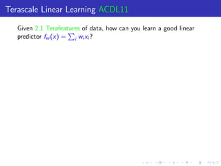
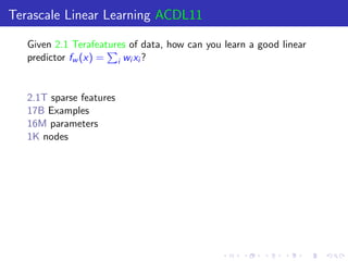
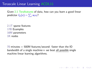
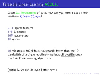
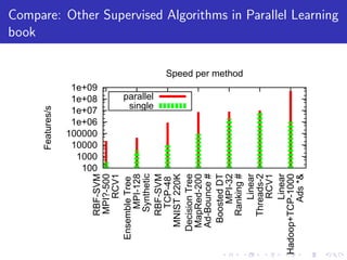
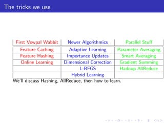
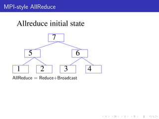
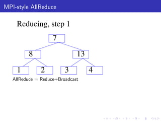
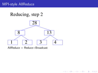
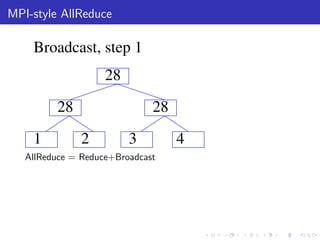
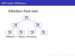
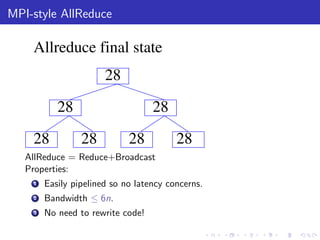
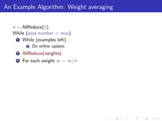
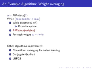
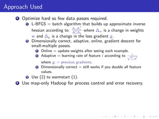
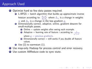
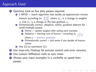
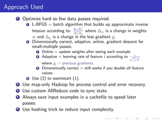
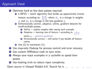
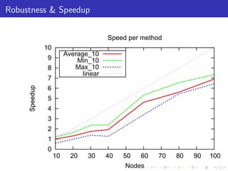
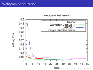
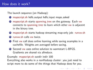
The document describes a terascale learning algorithm for training linear models on large datasets using distributed computing. It discusses using a hashing trick to reduce input complexity, an adaptive online gradient descent algorithm to warm-start L-BFGS batch optimization, and a custom all-reduce implementation to synchronize model parameters across nodes. The approach leverages Hadoop for fault tolerance while training linear models on up to 2.1 trillion features and 17 billion examples in 70 minutes, significantly faster than single machine algorithms.

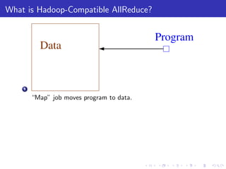
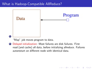
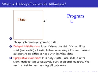
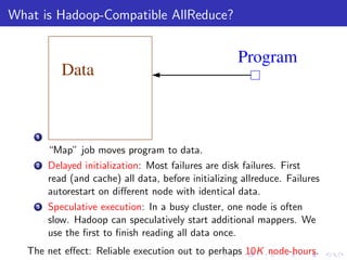


![[Harvard CS264] 09 - Machine Learning on Big Data: Lessons Learned from Googl...](https://cdn.slidesharecdn.com/ss_thumbnails/machinelearningbigdata-maxlin-cs264opt-110331195757-phpapp01-thumbnail.jpg?width=640&height=640&fit=bounds)


