The document provides an overview of reinforcement learning, detailing its components such as policies, reward signals, and value functions, alongside methodologies like temporal-difference learning and policy gradient methods. It discusses the exploration-exploitation trade-off in agent-environment interactions and highlights model-free versus model-based approaches, as well as various algorithms including Q-learning and deep Q-networks. Furthermore, the document touches on the importance of experience replay and the training of neural networks in deep reinforcement learning contexts.

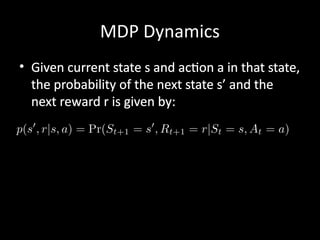
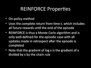
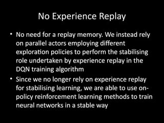
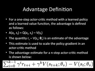
1. Reinforcement Learning
Karan Kathpalia

2. Overview
• Introduction to Reinforcement Learning
• Finite Markov Decision Processes
• Temporal-Difference Learning (SARSA, Q-
learning, Deep Q-Networks)
• Policy Gradient Methods (Finite Difference
Policy Gradient, REINFORCE, Actor-Critic)
• Asynchronous Reinforcement Learning

3. Introduction to Reinforcement
Learning
Chapter 1 – Reinforcement Learning: An Introduction
Imitation Learning Lecture Slides from CMU Deep
Reinforcement Learning Course

4. What is Reinforcement Learning?
• Learning from interaction with an environment to
achieve some long-term goal that is related to the
state of the environment
• The goal is defined by reward signal, which must be
maximised
• Agent must be able to partially/fully sense the
environment state and take actions to influence the
environment state
• The state is typically described with a feature-vector

5. Exploration versus Exploitation
• We want a reinforcement learning agent to earn lots of
reward
• The agent must prefer past actions that have been found to
be effective at producing reward
• The agent must exploit what it already knows to obtain
reward
• The agent must select untested actions to discover reward-
producing actions
• The agent must explore actions to make better action
selections in the future
• Trade-off between exploration and exploitation

6. Reinforcement Learning Systems
• Reinforcement learning systems have 4 main
elements:
– Policy
– Reward signal
– Value function
– Optional model of the environment

7. Policy
• A policy is a mapping from the perceived
states of the environment to actions to be
taken when in those states
• A reinforcement learning agent uses a policy
to select actions given the current
environment state

8. Reward Signal
• The reward signal defines the goal
• On each time step, the environment sends a
single number called the reward to the
reinforcement learning agent
• The agent’s objective is to maximise the total
reward that it receives over the long run
• The reward signal is used to alter the policy

9. Value Function (1)
• The reward signal indicates what is good in the short run
while the value function indicates what is good in the long
run
• The value of a state is the total amount of reward an agent
can expect to accumulate over the future, starting in that
state
• Compute the value using the states that are likely to follow
the current state and the rewards available in those states
• Future rewards may be time-discounted with a factor in
the interval [0, 1]

10. Value Function (2)
• Use the values to make and evaluate decisions
• Action choices are made based on value
judgements
• Prefer actions that bring about states of highest
value instead of highest reward
• Rewards are given directly by the environment
• Values must continually be re-estimated from the
sequence of observations that an agent makes
over its lifetime

11. Model-free versus Model-based
• A model of the environment allows inferences to be made about
how the environment will behave
• Example: Given a state and an action to be taken while in that state,
the model could predict the next state and the next reward
• Models are used for planning, which means deciding on a course of
action by considering possible future situations before they are
experienced
• Model-based methods use models and planning. Think of this as
modelling the dynamics p(s’ | s, a)
• Model-free methods learn exclusively from trial-and-error (i.e. no
modelling of the environment)
• This presentation focuses on model-free methods

12. On-policy versus Off-policy
• An on-policy agent learns only about the
policy that it is executing
• An off-policy agent learns about a policy or
policies different from the one that it is
executing

13. Credit Assignment Problem
• Given a sequence of states and actions, and the
final sum of time-discounted future rewards,
how do we infer which actions were effective at
producing lots of reward and which actions
were not effective?
• How do we assign credit for the observed
rewards given a sequence of actions over time?
• Every reinforcement learning algorithm must
address this problem

14. Reward Design
• We need rewards to guide the agent to achieve its
goal
• Option 1: Hand-designed reward functions
• This is a black art
• Option 2: Learn rewards from demonstrations
• Instead of having a human expert tune a system
to achieve the desired behaviour, the expert can
demonstrate desired behaviour and the robot can
tune itself to match the demonstration

15. What is Deep Reinforcement Learning?
• Deep reinforcement learning is standard reinforcement learning
where a deep neural network is used to approximate either a
policy or a value function
• Deep neural networks require lots of real/simulated interaction
with the environment to learn
• Lots of trials/interactions is possible in simulated environments
• We can easily parallelise the trials/interaction in simulated
environments
• We cannot do this with robotics (no simulations) because action
execution takes time, accidents/failures are expensive and there
are safety concerns

16. Finite Markov Decision Processes
Chapter 3 – Reinforcement Learning: An Introduction

17. Markov Decision Process (MDP)
• Set of states S
• Set of actions A
• State transition probabilities p(s’ | s, a). This is the
probability distribution over the state space given
we take action a in state s
• Discount factor γ in [0, 1]
• Reward function R: S x A -> set of real numbers
• For simplicity, assume discrete rewards
• Finite MDP if both S and A are finite

18. Time Discounting
• The undiscounted formulation γ = 0 across episodes is
appropriate for episodic tasks in which agent-environment
interaction breaks into episodes (multiple trials to perform a
task).
• Example: Playing Breakout (each run of the game is an
episode)
• The discounted formulation 0 < γ <= 1 is appropriate for
continuing tasks, in which the interaction continues without
limit
• Example: Vacuum cleaner robot
• This presentation focuses on episodic tasks

19. Agent-Environment Interaction (1)
• The agent and environment interact at each of a
sequence of discrete time steps t = {0, 1, 2, 3, …,
T} where T can be infinite
• At each time step t, the agent receives some
representation of the environment state St in S
and uses this to select an action At in the set A(St)
of available actions given that state
• One step later, the agent receives a numerical
reward Rt+1 and finds itself in a new state St+1

20. Agent-Environment Interaction (2)
• At each time step, the agent implements a
stochastic policy or mapping from states to
probabilities of selecting each possible action
• The policy is denoted πt where πt(a | s) is the
probability of taking action a when in state s
• A policy is a stochastic rule by which the agent
selects actions as a function of states
• Reinforcement learning methods specify how the
agent changes its policy using its experience

21. Action Selection
• At time t, the agent tries to select an action to
maximise the sum Gt of discounted rewards
received in the future

22. MDP Dynamics
• Given current state s and action a in that state,
the probability of the next state s’ and the
next reward r is given by:

23. State Transition Probabilities
• Suppose the reward function is discrete and
maps from S x A to W
• The state transition probability or probability
of transitioning to state s’ given current state s
and action a in that state is given by:

24. Expected Rewards
• The expected reward for a given state-action
pair is given by:

25. State-Value Function (1)
• Value functions are defined with respect to
particular policies because future rewards
depend on the agent’s actions
• Value functions give the expected return of a
particular policy
• The value vπ(s) of a state s under a policy π is
the expected return when starting in state s and
following the policy π from that state onwards

26. State-Value Function (2)
• The state-value function vπ(s) for the policy π
is given below. Note that the value of the
terminal state (if any) is always zero.

27. Action-Value Function
• The value qπ(s, a) of taking action a in state s
under a policy π is defined as the expected
return starting from s, taking the action a and
thereafter following policy π
• qπ is the action-value function for policy π

28. Bellman Equation (1)
• The equation expresses the relationship
between the value of a state s and the values
of its successor states
• The value of the next state must equal the
discounted value of the expected next state,
plus the reward expected along the way

29. Bellman Equation (2)
• The value of state s is the expected value of
the sum of time-discounted rewards (starting
at current state) given current state s
• This is expected value of r plus the sum of
time-discounted rewards (starting at successor
state) over all successor states s’ and all next
rewards r and over all possible actions a in
current state s

30. Optimality
• A policy is defined to be better than or equal to another
policy if its expected return is greater than or equal to that
of the other policy for all states
• There is always at least one optimal policy π* that is better
than or equal to all other policies
• All optimal policies share the same optimal state-value
function v*, which gives the maximum expected return for
any state s over all possible policies
• All optimal policies share the same optimal action-value
function q*, which gives the maximum expected return for
any state-action pair (s, a) over all possible policies

31. Temporal-Difference Learning
Chapter 6 – Reinforcement Learning: An Introduction
Playing Atari with Deep Reinforcement Learning
Asynchronous Methods for Deep Reinforcement Learning
David Silver’s Tutorial on Deep Reinforcement Learning

32. What is TD learning?
• Temporal-Difference learning = TD learning
• The prediction problem is that of estimating the value
function for a policy π
• The control problem is the problem of finding an optimal
policy π*
• Given some experience following a policy π, update estimate
v of vπ for non-terminal states occurring in that experience
• Given current step t, TD methods wait until the next time
step to update V(St)
• Learn from partial returns

33. Value-based Reinforcement Learning
• We want to estimate the optimal value V*(s) or
action-value function Q*(s, a) using a function
approximator V(s; θ) or Q(s, a; θ) with
parameters θ
• This function approximator can be any
parametric supervised machine learning model
• Recall that the optimal value is the maximum
value achievable under any policy

34. Update Rule for TD(0)
• At time t + 1, TD methods immediately form a
target Rt+1 + γ V(St+1) and make a useful update
with step size α using the observed reward Rt+1
and the estimate V(St+1)
• The update is the step size times the
difference between the target output and the
actual output

35. Update Rule Intuition
• The target output is a more accurate estimate of
V(St) given the reward Rt+1 is known
• The actual output is our current estimate of V(St)
• We simply take one step with our current value
function estimate to get a more accurate
estimate of V(St) and then perform an update to
move V(St) closer towards the more accurate
estimate (i.e. temporal difference)

36. Tabular TD(0) Algorithm

37. SARSA – On-policy TD Control
• SARSA = State-Action-Reward-State-Action
• Learn an action-value function instead of a
state-value function
• qπ is the action-value function for policy π
• Q-values are the values qπ(s, a) for s in S, a in A
• SARSA experiences are used to update Q-
values
• Use TD methods for the prediction problem

38. SARSA Update Rule
• We want to estimate qπ(s, a) for the current policy π,
and for all states s and action a
• The update rule is similar to that for TD(0) but we
transition from state-action pair to state-action pair,
and learn the values of state-action pairs
• The update is performed after every transition from
a non-terminal state St
• If St+1 is terminal, then Q(St+1, At+1) is zero
• The update rule uses (St, At, Rt+1, St+1, At+1)

39. SARSA Algorithm

40. Q-learning – Off-policy TD Control
• Similar to SARSA but off-policy updates
• The learned action-value function Q directly approximates
the optimal action-value function q* independent of the
policy being followed
• In update rule, choose action a that maximises Q given St+1
and use the resulting Q-value (i.e. estimated value given by
optimal action-value function) plus the observed reward as
the target
• This method is off-policy because we do not have a fixed
policy that maps from states to actions. This is why At+1 is not
used in the update rule

41. One-step Q-learning Algorithm

42. Epsilon-greedy Policy
• At each time step, the agent selects an action
• The agent follows the greedy strategy with
probability 1 – epsilon
• The agent selects a random action with
probability epsilon
• With Q-learning, the greedy strategy is the
action a that maximises Q given St+1

43. Deep Q-Networks (DQN)
• Introduced deep reinforcement learning
• It is common to use a function approximator Q(s, a; θ)
to approximate the action-value function in Q-learning
• Deep Q-Networks is Q-learning with a deep neural
network function approximator called the Q-network
• Discrete and finite set of actions A
• Example: Breakout has 3 actions – move left, move
right, no movement
• Uses epsilon-greedy policy to select actions

44. Q-Networks
• Core idea: We want the neural network to learn a
non-linear hierarchy of features or feature
representation that gives accurate Q-value
estimates
• The neural network has a separate output unit for
each possible action, which gives the Q-value
estimate for that action given the input state
• The neural network is trained using mini-batch
stochastic gradient updates and experience replay

45. Experience Replay
• The state is a sequence of actions and
observations st = x1, a1, x2, …, at-1, xt
• Store the agent’s experiences at each time step
et = (st, at, rt, st+1) in a dataset D = e1, ..., en pooled
over many episodes into a replay memory
• In practice, only store the last N experience
tuples in the replay memory and sample
uniformly from D when performing updates

46. State representation
• It is difficult to give the neural network a
sequence of arbitrary length as input
• Use fixed length representation of
sequence/history produced by a function ϕ(st)
• Example: The last 4 image frames in the
sequence of Breakout gameplay

47. Q-Network Training
• Sample random mini-batch of experience tuples
uniformly at random from D
• Similar to Q-learning update rule but:
– Use mini-batch stochastic gradient updates
– The gradient of the loss function for a given iteration with
respect to the parameter θi is the difference between the
target value and the actual value is multiplied by the gradient
of the Q function approximator Q(s, a; θ) with respect to that
specific parameter
• Use the gradient of the loss function to update the Q
function approximator

48. Loss Function Gradient Derivation

49. DQN Algorithm

50. Comments
• It was previously thought that the combination of simple online
reinforcement learning algorithms with deep neural networks was
fundamentally unstable
• The sequence of observed data (states) encountered by an online
reinforcement learning agent is non-stationary and online updates are
strongly correlated
• The technique of DQN is stable because it stores the agent’s data in
experience replay memory so that it can be randomly sampled from
different time-steps
• Aggregating over memory reduces non-stationarity and decorrelates
updates but limits methods to off-policy reinforcement learning algorithms
• Experience replay updates use more memory and computation per real
interaction than online updates, and require off-policy learning algorithms
that can update from data generated by an older policy

51. Policy Gradient Methods
Chapter 13 – Reinforcement Learning: An Introduction
Policy Gradient Lecture Slides from David Silver’s Reinforcement
Learning Course
David Silver’s Tutorial on Deep Reinforcement Learning

52. What are Policy Gradient Methods?
• Before: Learn the values of actions and then select actions based
on their estimated action-values. The policy was generated
directly from the value function
• We want to learn a parameterised policy that can select actions
without consulting a value function. The parameters of the policy
are called policy weights
• A value function may be used to learn the policy weights but this
is not required for action selection
• Policy gradient methods are methods for learning the policy
weights using the gradient of some performance measure with
respect to the policy weights
• Policy gradient methods seek to maximise performance and so
the policy weights are updated using gradient ascent

53. Policy-based Reinforcement Learning
• Search directly for the optimal policy π*
• Can use any parametric supervised machine
learning model to learn policies π(a |s; θ)
where θ represents the learned parameters
• Recall that the optimal policy is the policy that
achieves maximum future return

54. Notation
• Policy weight vector θ
• The policy is π(a | s, θ), which represents the probability
that action a is taken in state s with policy weight vector
θ
• If using learned value functions, the value function’s
weight vector is w
• Performance measure η(θ)
• Episodic case: η(θ) = vπ(s0)
• Performance is defined as the value of the start state
under the parameterised policy

55. Policy Approximation
• The policy can be parameterised in any way provided π(a | s,
θ) is differentiable with respect to its weights
• To ensure exploration, we generally require that the policy
never becomes deterministic and so π(a | s, θ) is in interval
(0, 1)
• Assume discrete and finite set of actions
• Form parameterised numerical preferences h(s, a, θ) for each
state-action pair
• Can use a deep neural network as the policy approximator
• Use softmax so that the most preferred actions in each state
are given the highest probability of being selected

56. Types of Policy Gradient Method
• Finite Difference Policy Gradient
• Monte Carlo Policy Gradient
• Actor-Critic Policy Gradient

57. Finite Difference Policy Gradient
• Compute the partial derivative of the performance measure η(θ) with
respect to θk using finite difference gradient approximation
• Compute performance measure η(θ)
• Perturb θ by small positive amount epsilon in the kth dimension and
compute performance measure η(θ + ukε) where uk is unit vector that
is 1 in kth component and 0 elsewhere
• The partial derivative is approximated by
( η(θ + ukε) - η(θ) ) / ε
• θk <- θk + α ( η(θ + ukε) - η(θ) ) / ε
• Perform gradient ascent using the partial derivative
• Simple, noisy and inefficient procedure that is sometimes effective
• This procedure works for arbitrary policies (can be non-differentiable)

58. REINFORCE: Monte Carlo Policy Gradient
• We want a quantity that we can sample on
each time step whose expectation is equal to
the gradient
• We can then perform stochastic gradient
ascent with this quantity

59. REINFORCE Properties
• On-policy method
• Uses the complete return from time t, which includes
all future rewards until the end of the episode
• REINFORCE is thus a Monte Carlo algorithm and is
only well-defined for the episodic case with all
updates made in retrospect after the episode is
completed
• Note that the gradient of log x is the gradient of x
divided by x by the chain rule

60. REINFORCE Algorithm

61. Actor-Critic Methods
• Methods that learn approximations to both policy and
value functions are called actor-critic methods
• Actor refers to the learned policy
• Critic refers to the learned value function, which is
usually a state-value function
• The critic is bootstrapped – the state-values are
updated using the estimated state-values of
subsequent states
• The number of steps in the actor-critic method
controls the degree of bootstrapping

62. One-step Actor-Critic Update Rules
• On-policy method
• The state-value function update rule is the TD(0) update
rule
• The policy function update rule is shown below.
• For n-step Actor-Critic, simply replace Gt
(1)
with Gt
(n)

63. One-step Actor-Critic Algorithm

64. Asynchronous Reinforcement
Learning
Asynchronous Methods for Deep Reinforcement Learning

65. What is Asynchronous Reinforcement Learning?
• Use asynchronous gradient descent to optimise
controllers
• This is useful for deep reinforcement learning
where the controllers are deep neural networks,
which take a long time to train
• Asynchronous gradient descent speeds up the
learning process
• Can use one multi-core CPU to train deep neural
networks asynchronously instead of multiple GPUs

66. Parallelism (1)
• Asynchronously execute multiple agents in parallel on multiple
instances of the environment
• This parallelism decorrelates the agents’ data into a more
stationary process since at any given time-step, the agents will be
experiencing a variety of different states
• This approach enables a larger spectrum of fundamental on-
policy and off-policy reinforcement learning algorithms to be
applied robustly and effectively using deep neural networks
• Use asynchronous actor-learners (i.e. agents). Think of each actor-
learner as a thread
• Run everything on a single multi-core CPU to avoid
communication costs of sending gradients and parameters

67. Parallelism (2)
• Multiple actor-learners running in parallel are likely
to be exploring different parts of the environment
• We can explicitly use different exploration policies
in each actor-learner to maximise this diversity
• By running different exploration policies in
different threads, the overall changes made to the
parameters by multiple actor-learners applying
updates in parallel are less likely to be correlated in
time than a single agent applying online updates

68. No Experience Replay
• No need for a replay memory. We instead rely
on parallel actors employing different
exploration policies to perform the stabilising
role undertaken by experience replay in the
DQN training algorithm
• Since we no longer rely on experience replay
for stabilising learning, we are able to use on-
policy reinforcement learning methods to train
neural networks in a stable way

69. Asynchronous Algorithms
• Asynchronous one-step Q-learning
• Asynchronous one-step SARSA
• Asynchronous n-step Q-learning
• Asynchronous Advantage Actor-Critic (A3C)

70. Asynchronous one-step Q-learning
• Each thread interacts with its own copy of the environment
and at each step, computes the gradient of the Q-learning
loss
• Use a globally shared and slowly changing target network
with parameters θ-
when computing the Q-learning loss
• DQN uses a globally shared and slowly changing target
network too – the network is updated using a mini-batch of
experience tuples drawn from replay memory
• The gradients are accumulated over multiple time-steps
before being applied (similar to using mini-batches), which
reduces chance of multiple actor-learners overwriting each
other’s updates

71. Exploration
• Giving each thread a different exploration
policy helps improve robustness and generally
improves performance through better
exploration
• Use epsilon-greedy exploration with epsilon
periodically sampled from some distribution
by each thread

72. Asynchronous one-step Q-learning Algorithm

73. Asynchronous one-step SARSA
• This is the same algorithm as Asynchronous
one-step Q-learning except the target value
used for Q(s, a) is different
• One-step SARSA uses r + γ Q(s’, a’; θ-
) as the
target value

74. n-step Q-learning
• So far we have been using one-step Q-learning
• One-step Q-learning updates the action value Q(s, a) towards r
+ γ maxa’ Q(s’, a’; θ), which is the one-step return
• Obtaining a reward r only directly affects the value of the state-
action pair (s, a) that led to the reward
• The values of the other state-action pairs are affected only
indirectly through the updated value Q(s, a)
• This can make the learning process slow since many updates
are required to propagate a reward to the relevant preceding
states and actions
• Use n-step returns to propagate the rewards faster

75. n-step Returns
• In n-step Q-learning, Q(s, a) is updated towards the n-step
return:
• rt + γ rt+1 + … + γn-1
rt+n-1 + maxa γn
Q(st+n, a)
• This results in a single reward directly affecting the values of
n preceding state-action pairs
• This makes the process of propagating rewards to relevant
state-action pairs potentially much more efficient
• One-step update for the last state, two-step update for the
second last state, and so on until n-step update for the nth
last state
• Accumulated updates are applied in a single step

76. Asynchronous n-step Q-learning Algorithm

77. A3C
• Maintains a policy π(at| st; θ) and an estimate of the
value function V(st; θv)
• n-step Actor-Critic method
• As with value-based methods, use parallel actor-learners
and accumulate updates to improve training stability
• In practice, the policy approximation and the value
function share some parameters
• Use a neural network that has one softmax output for the
policy π(at| st; θ) and one linear output for the value
function V(st; θv) with all non-output parameters shared

78. Advantage Definition
• For a one-step actor-critic method with a learned policy
and a learned value function, the advantage is defined
as follows:
• A(at, st) = Q(at, st) – V(st)
• The quantity rt – V(st; θv) is an estimate of the advantage
• This estimate is used to scale the policy gradient in an
actor-critic method
• The advantage estimate for a n-step actor-critic method
is shown below:

79. A3C Algorithm

80. Summary
• Get faster training because of parallelism
• Can use on-policy reinforcement learning
methods
• Diversity in exploration can lead to better
performance than synchronous methods
• In practice, the on-policy A3C algorithm appears
to be the best performing asynchronous
reinforcement learning method in terms of
performance and training speed