Download as PDF, PPTX
![241-306 Discrete-Time Fourier Transform
3
Development of the Fourier Transform
Representation of an Aperiodic Signal
1 The Representation of Aperiodic Signals : The
Discrete-Time Fourier Transform
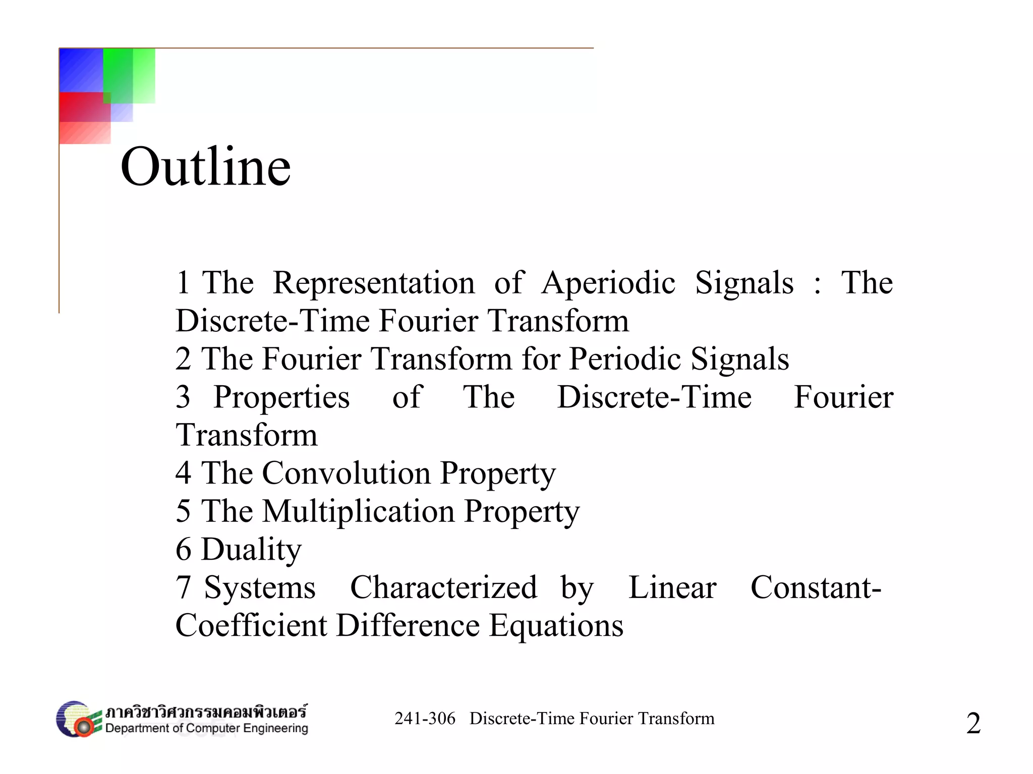
Consider a sequence x[n] that is of finite duration and
x[n] = 0 outside the range -N1
≤ n ≤ N2
. From the
aperiodic signal, we can construct a periodic
sequence when x[n] is one periodx[n]
x[n]= ∑
k=〈N 〉
ak e jk2/ N n](https://image.slidesharecdn.com/chapter51-200511110125/75/Chapter5-The-Discrete-Time-Fourier-Transform-3-2048.jpg)
![241-306 Discrete-Time Fourier Transform
5
ak=
1
N
∑
n=〈N 〉
x[n]e− jk 2/N n
ak=
1
N
∑
n=−N1
N 2
x[n]e− jk 2/N n
=
1
N
∑
n=−∞
∞
x[n]e− jk 2/N n
Since for -N1
≤ n ≤ N2
, and also,
x[n] = 0 outside this interval
x[n]=x[n]](https://image.slidesharecdn.com/chapter51-200511110125/75/Chapter5-The-Discrete-Time-Fourier-Transform-5-2048.jpg)
![241-306 Discrete-Time Fourier Transform
6
X e j
= ∑
n=−∞
∞
x[n]e− jn
ak=
1
N
X e
jk 0
x[n]= ∑
k=〈N 〉
1
N
X e
jk 0
e
jk 0 n
Defining the function
we have
we can express](https://image.slidesharecdn.com/chapter51-200511110125/75/Chapter5-The-Discrete-Time-Fourier-Transform-6-2048.jpg)
![241-306 Discrete-Time Fourier Transform
7
x[n]=
1
2
∑
k=〈 N 〉
X e
jk 0
e
jk 0 n
0
since 2π/N = ω0
ω → 0 as N→ ∞, the right-hand side passes to
integral.](https://image.slidesharecdn.com/chapter51-200511110125/75/Chapter5-The-Discrete-Time-Fourier-Transform-7-2048.jpg)
![241-306 Discrete-Time Fourier Transform
8
x[n]=
1
2
∫
2
X e j
e jn
d
X e
j
= ∑
n=−∞
∞
x[n]e
− jn
Fourier Transform pair
Inverse Fourier Transform(synthesis equation)
Fourier Transform (analysis equation)](https://image.slidesharecdn.com/chapter51-200511110125/75/Chapter5-The-Discrete-Time-Fourier-Transform-8-2048.jpg)
![241-306 Discrete-Time Fourier Transform
11
Example 5.1
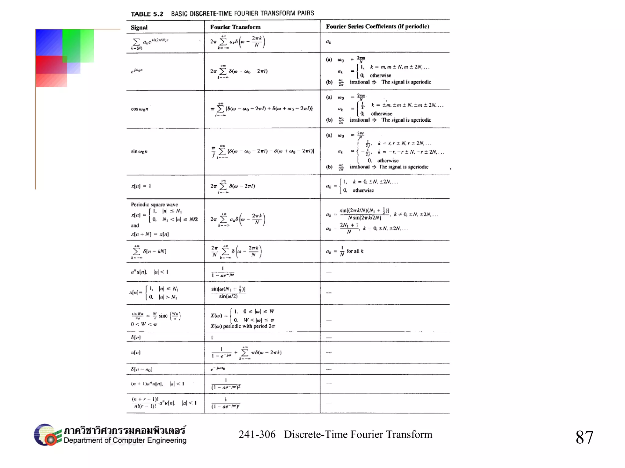
x[n]=a
n
u[n], ∣a∣1
X e j
= ∑
n=−∞
∞
an
u[n]e− jn
=∑
n=0
∞
ae
− j
n
=
1
1−ae
− j
Find the Fourier Transform for the signal
solution](https://image.slidesharecdn.com/chapter51-200511110125/75/Chapter5-The-Discrete-Time-Fourier-Transform-11-2048.jpg)
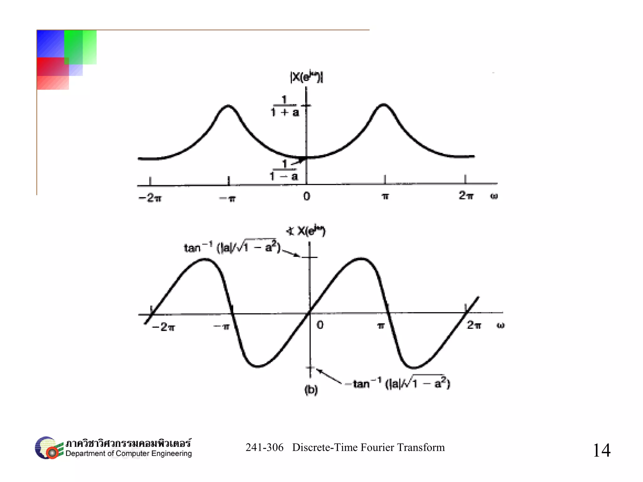
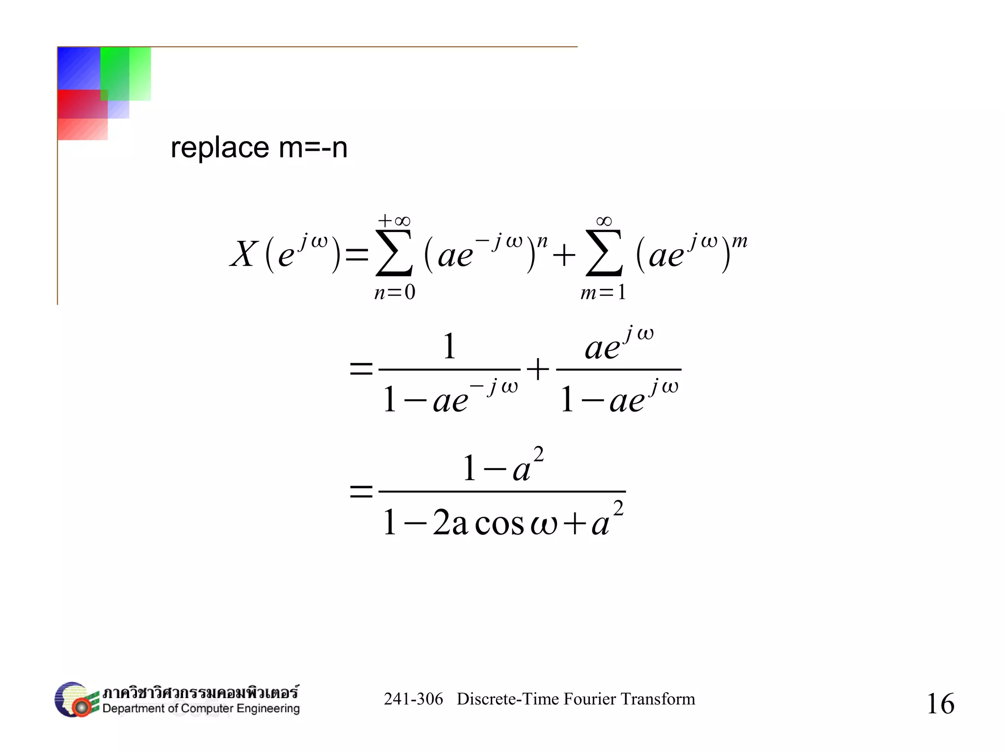
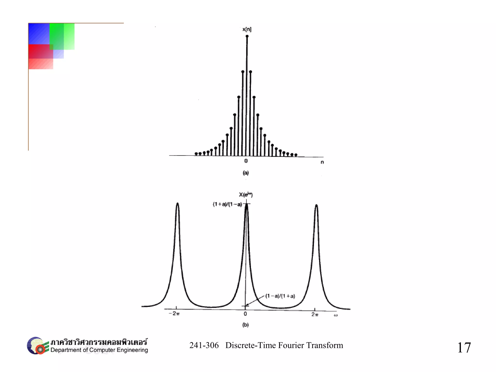
![241-306 Discrete-Time Fourier Transform
15
Example 5.2
x[n]=a
∣n∣
, ∣a∣1
X e j
= ∑
n=−∞
∞
a∣n∣
e− j n
Find the Fourier Transform for the signal
solution
=∑
n=0
∞
an
e− jn
∑
n=−∞
−1
a−n
e− jn](https://image.slidesharecdn.com/chapter51-200511110125/75/Chapter5-The-Discrete-Time-Fourier-Transform-15-2048.jpg)
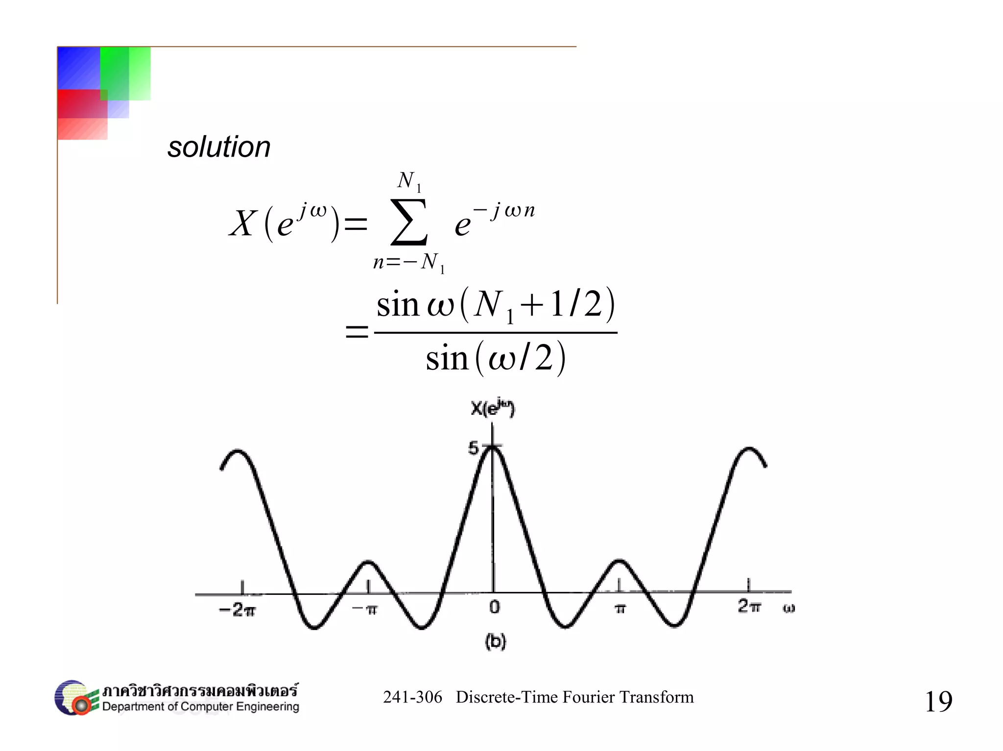
![241-306 Discrete-Time Fourier Transform
18
Example 5.3
Find the Fourier Transform for the signal
x[n]=
{1, ∣n∣≤N1
0, ∣n∣N1](https://image.slidesharecdn.com/chapter51-200511110125/75/Chapter5-The-Discrete-Time-Fourier-Transform-18-2048.jpg)
![241-306 Discrete-Time Fourier Transform
20
Convergence of Fourier Transforms
∑
n=−∞
∞
∣x[n]∣2
∞
if the sequence x[n] has finite energy
we guaranteed that X(ejω
) is finite
∑
n=−∞
∞
∣x[n]∣∞
The condition on x[n] that guarantee the
convergence of Fourier transform is](https://image.slidesharecdn.com/chapter51-200511110125/75/Chapter5-The-Discrete-Time-Fourier-Transform-20-2048.jpg)
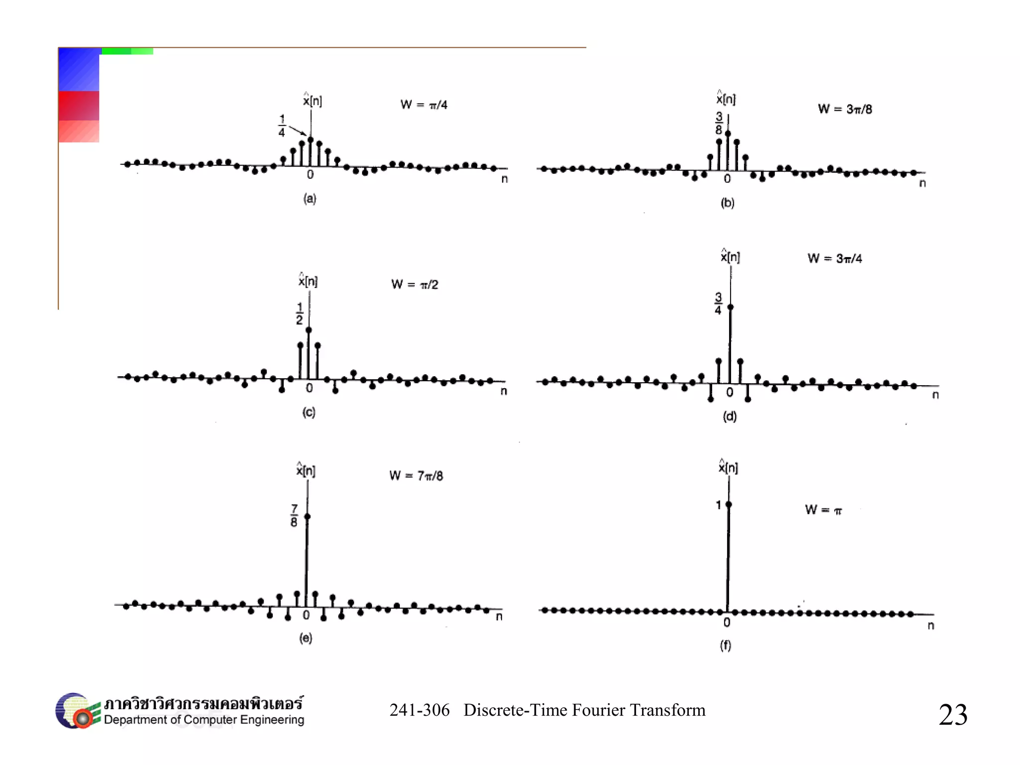
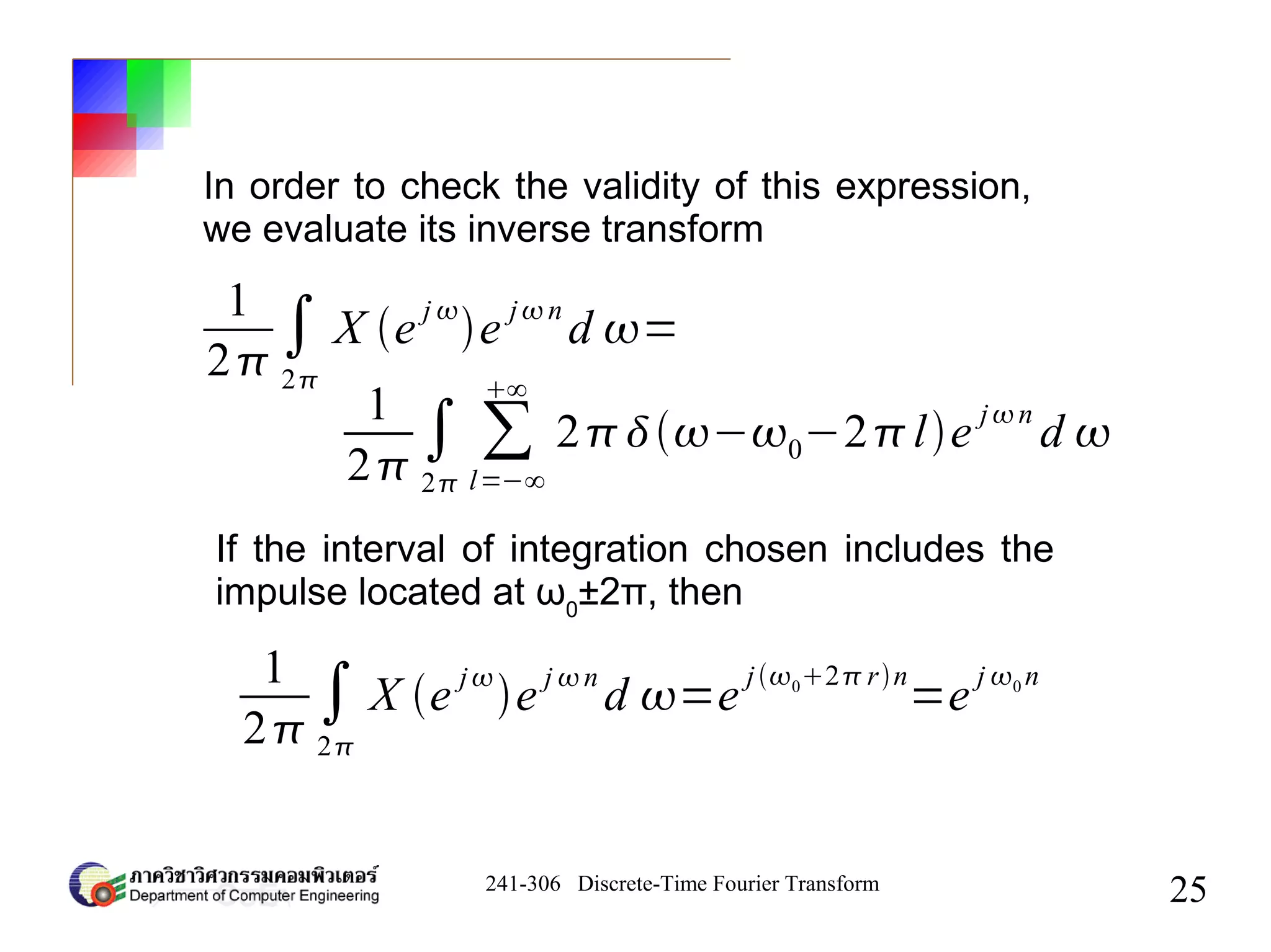
![241-306 Discrete-Time Fourier Transform
21
There are no convergence issues associated with
the synthesis equation, since the integral in this
equation is over a finite interval of integration.
x[n]=
1
2
∫
−W
W
X e j
e jn
d
x[n]
If we approximate an aperiodic signal x[n] by an
integral
then = x[n] for W = π](https://image.slidesharecdn.com/chapter51-200511110125/75/Chapter5-The-Discrete-Time-Fourier-Transform-21-2048.jpg)
![241-306 Discrete-Time Fourier Transform
22
Example 5.4
Let x[n] be the unit impulse
x[n]=[n]
X e j
=1
Fourier transform of this signal is
x[n]=
1
2
∫
−W
W
e
jn
d =
sinWn
n
We can approximate x[n] by](https://image.slidesharecdn.com/chapter51-200511110125/75/Chapter5-The-Discrete-Time-Fourier-Transform-22-2048.jpg)
![241-306 Discrete-Time Fourier Transform
24
2 The Fourier Transform for Periodic Signals
X e
j
= ∑
l=−∞
∞
2−0−2l
Let a signal x[n] is x[n]=e
j
0
n
The Fourier transform of x[n] should have
impulse at ω0
, ω0
±2π, ω0
±4π and so on](https://image.slidesharecdn.com/chapter51-200511110125/75/Chapter5-The-Discrete-Time-Fourier-Transform-24-2048.jpg)
![241-306 Discrete-Time Fourier Transform
26
X e j
= ∑
k=−∞
∞
2ak −
2k
N
x[n]= ∑
k=〈N 〉
ak e jk2/ N n
Consider a periodic sequence x[n] with period N
and with the Fourier series representation
The Fourier transform is](https://image.slidesharecdn.com/chapter51-200511110125/75/Chapter5-The-Discrete-Time-Fourier-Transform-26-2048.jpg)
![241-306 Discrete-Time Fourier Transform
27
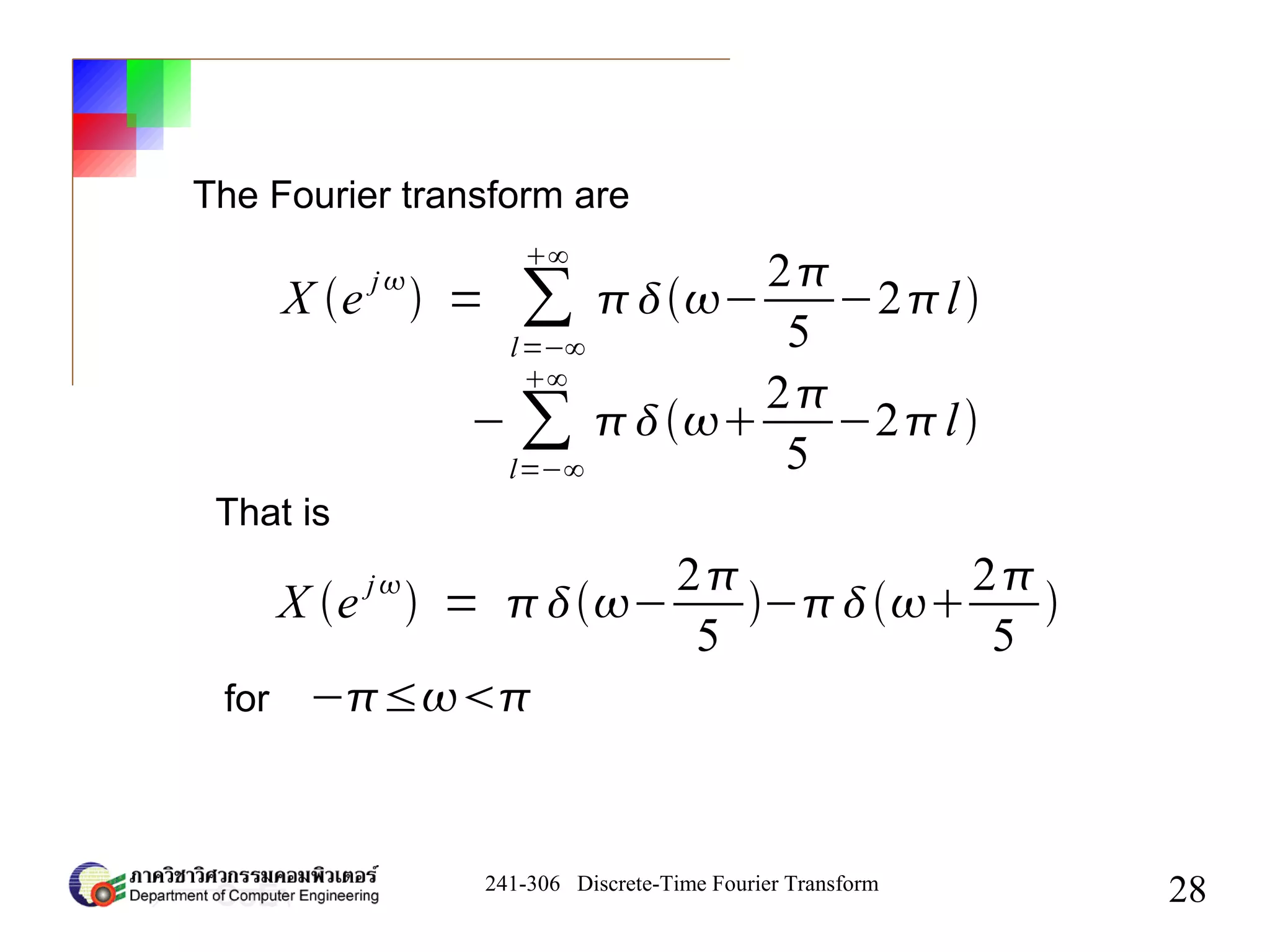
Example 5.5
Find Fourier transform of the signal
Solution
By Euler's relation
x[n]=cos0 n
x[n]=
1
2
e
j 0 n
1
2
e
− j 0 n
with 0=
2
5](https://image.slidesharecdn.com/chapter51-200511110125/75/Chapter5-The-Discrete-Time-Fourier-Transform-27-2048.jpg)
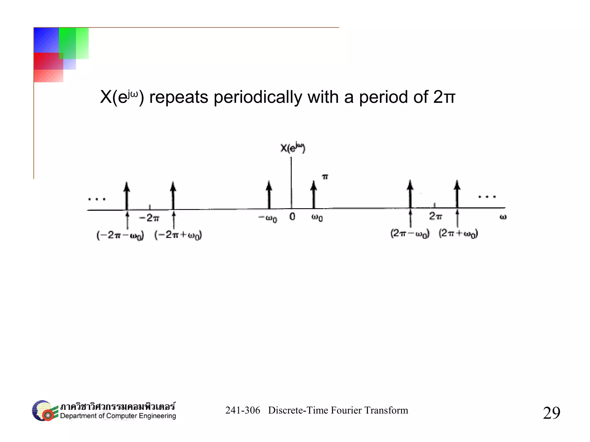
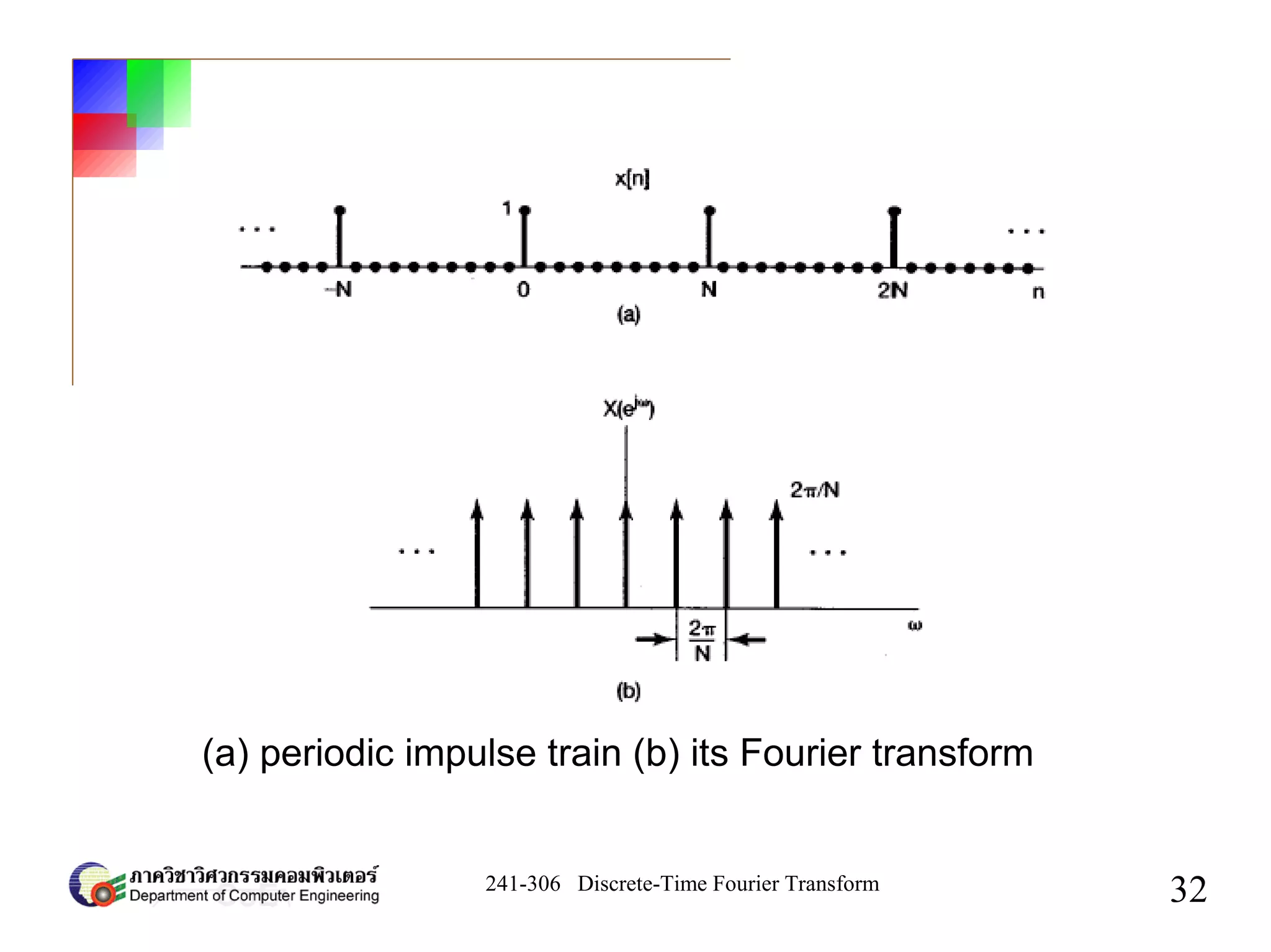
![241-306 Discrete-Time Fourier Transform
30
Example 5.6
x[n]= ∑
k=−∞
∞
n−kN
Find The Fourier transform of the impulse train](https://image.slidesharecdn.com/chapter51-200511110125/75/Chapter5-The-Discrete-Time-Fourier-Transform-30-2048.jpg)
![241-306 Discrete-Time Fourier Transform
31
Solution
ak=
1
N
∑
n=〈N 〉
x[n]e
− j k 2/ N n
=
1
N
X e j
=
2
N
∑
k=−∞
∞
−
2k
N
The Fourier series coefficients(for 0≤n≤N-1) are
given by
The Fourier transform given by](https://image.slidesharecdn.com/chapter51-200511110125/75/Chapter5-The-Discrete-Time-Fourier-Transform-31-2048.jpg)
![241-306 Discrete-Time Fourier Transform
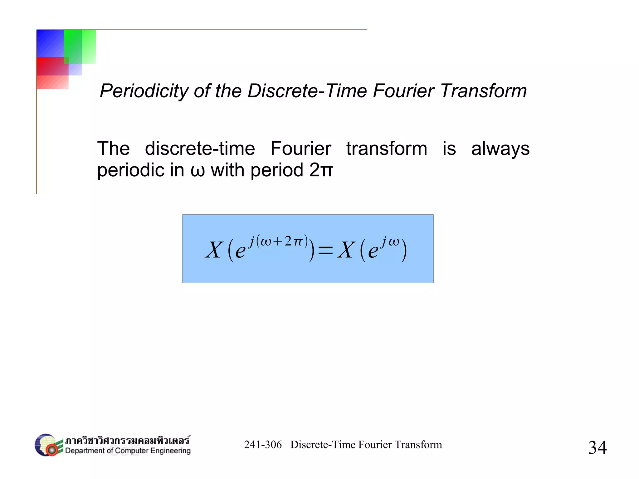
33
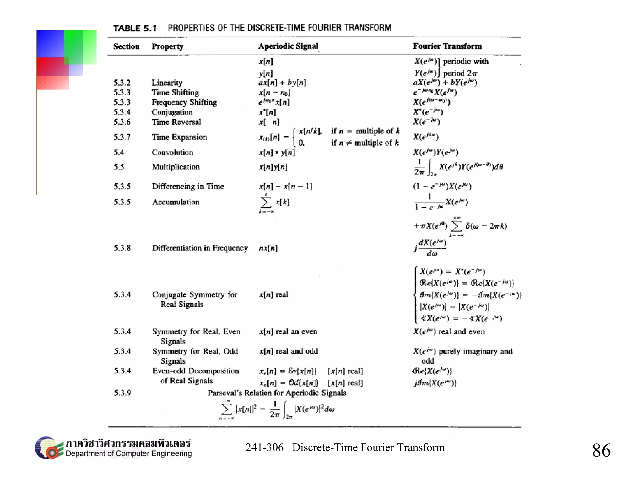
3 Properties of the Discrete-Time Fourier Transform
Notation x[n] ↔
F
X e
j
X e j
=F {x[n]}
x[n]=F
−1
{X e
j
}](https://image.slidesharecdn.com/chapter51-200511110125/75/Chapter5-The-Discrete-Time-Fourier-Transform-33-2048.jpg)
![241-306 Discrete-Time Fourier Transform
35
Linearity
x1[n] ↔
F
X 1e
j
x2[n] ↔
F
X 2 e
j
ax1[n]bx2[n] ↔
F
aX 1e
j
bX 2e
j
If
then](https://image.slidesharecdn.com/chapter51-200511110125/75/Chapter5-The-Discrete-Time-Fourier-Transform-35-2048.jpg)
![241-306 Discrete-Time Fourier Transform
36
Time Shifting and Frequency Shifting
x[n] ↔
F
X e
j
x[n−n0] ↔
F
e
− jn0
X e
j
If
then
e
− j 0 n
x[n] ↔
F
X e
j−0
and](https://image.slidesharecdn.com/chapter51-200511110125/75/Chapter5-The-Discrete-Time-Fourier-Transform-36-2048.jpg)
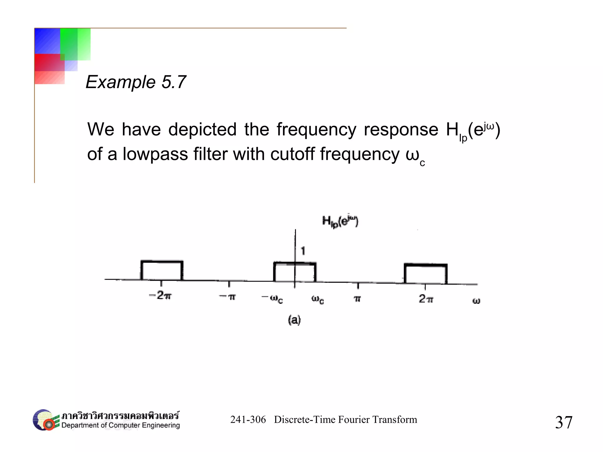
![241-306 Discrete-Time Fourier Transform
39
by the frequency-shifting property
hhp=e j n
hlp[n]
=−1n
hlp[n]](https://image.slidesharecdn.com/chapter51-200511110125/75/Chapter5-The-Discrete-Time-Fourier-Transform-39-2048.jpg)
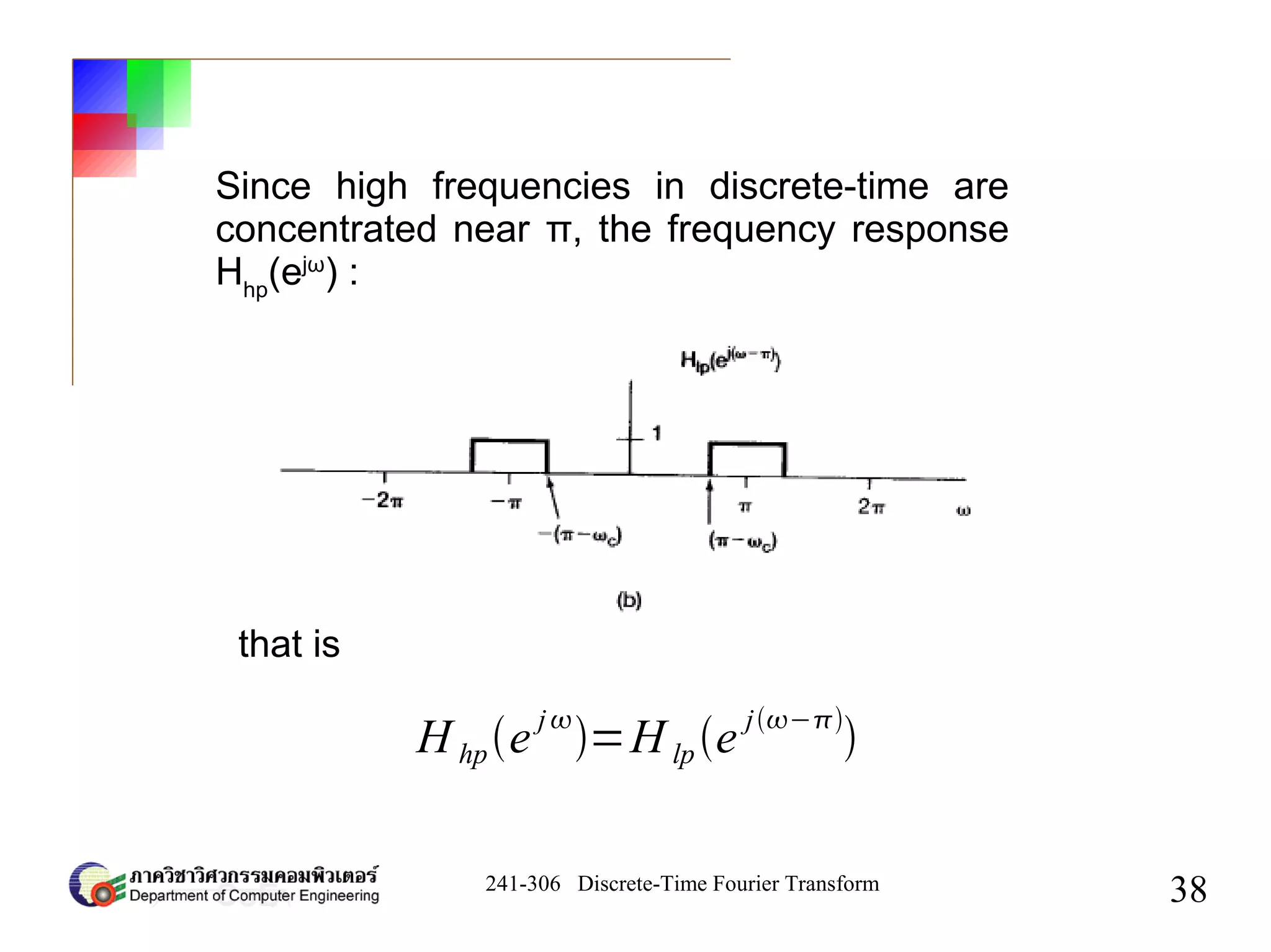
![241-306 Discrete-Time Fourier Transform
40
Conjugation and Conjugate Symmetry
x[n] ↔
F
X e
j
x
∗
[n] ↔
F
X
∗
e
− j
If
then](https://image.slidesharecdn.com/chapter51-200511110125/75/Chapter5-The-Discrete-Time-Fourier-Transform-40-2048.jpg)
![241-306 Discrete-Time Fourier Transform
41
Conjugate symmetry
If x[n] is real then X(ejω
) has conjugate symmetry
X e
− j
=X
∗
e
j
[x[n] real]
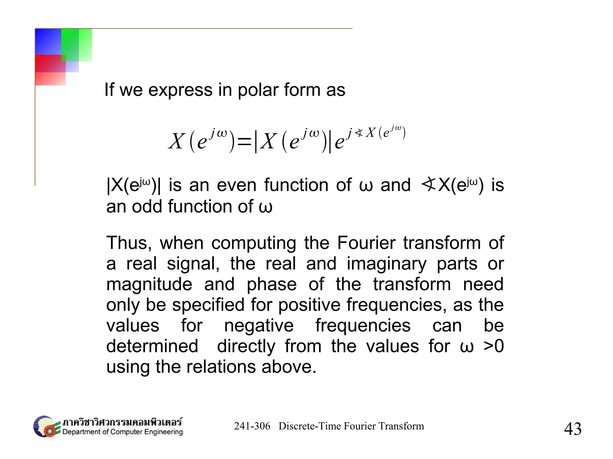
If we express X(ejω
) in rectangular form as
X e
j
=ℜe[ X e
j
] j ℑm[ X e
j
]](https://image.slidesharecdn.com/chapter51-200511110125/75/Chapter5-The-Discrete-Time-Fourier-Transform-41-2048.jpg)
![241-306 Discrete-Time Fourier Transform
42
then if x[n] is real
ℜe[ X e
j
]=ℜe[ X e
− j
]
ℑm[ X e
j
]=−ℑm[ X e
− j
]
and
The real part of Fourier transform is an even
function of frequency and the imaginary part is an
odd function of frequency](https://image.slidesharecdn.com/chapter51-200511110125/75/Chapter5-The-Discrete-Time-Fourier-Transform-42-2048.jpg)
![241-306 Discrete-Time Fourier Transform
44
If x[n] is real then it can always be expressed in
terms of the sum of an even function and an odd
function.
x[n]=xe [n]xo[n]
From the linearity property
F {x[n]}=F {xe[n]}F {xo[n]}
F {xe [n]} is a real function
F {xo [n]} is purely imaginary](https://image.slidesharecdn.com/chapter51-200511110125/75/Chapter5-The-Discrete-Time-Fourier-Transform-44-2048.jpg)
![241-306 Discrete-Time Fourier Transform
45
With x[n] real, we can conclude that
x[n] ↔
F
X e
j
Ev{x[n]} ↔
F
ℜe{X e
j
}
Od {x[n]} ↔
F
j ℑm{X e
j
}](https://image.slidesharecdn.com/chapter51-200511110125/75/Chapter5-The-Discrete-Time-Fourier-Transform-45-2048.jpg)
![241-306 Discrete-Time Fourier Transform
46
Differencing and Accumulation
Let x[n] be a signal with Fourier transform X(ejω
),
the Fourier transform pair for the first-difference
signal x[n]-x[n-1] is given by
x[n]−x[n−1] ↔
F
1−e
− j
X e
j
](https://image.slidesharecdn.com/chapter51-200511110125/75/Chapter5-The-Discrete-Time-Fourier-Transform-46-2048.jpg)
![241-306 Discrete-Time Fourier Transform
47
∑
m=−∞
n
x[m] ↔
F 1
1−e
− j
X e j
X e j0
∑
k=−∞
∞
−2k
Consider the signal
Since y[n] - y[n-1] = x[n] , we might conclude that
the transform of y[n] should be related to the
transform of x[n] by
y[n]= ∑
m=−∞
n
x[m]
The impulse train on the right-hand side reflects
the dc or average value that can result from
summation.](https://image.slidesharecdn.com/chapter51-200511110125/75/Chapter5-The-Discrete-Time-Fourier-Transform-47-2048.jpg)
![241-306 Discrete-Time Fourier Transform
48
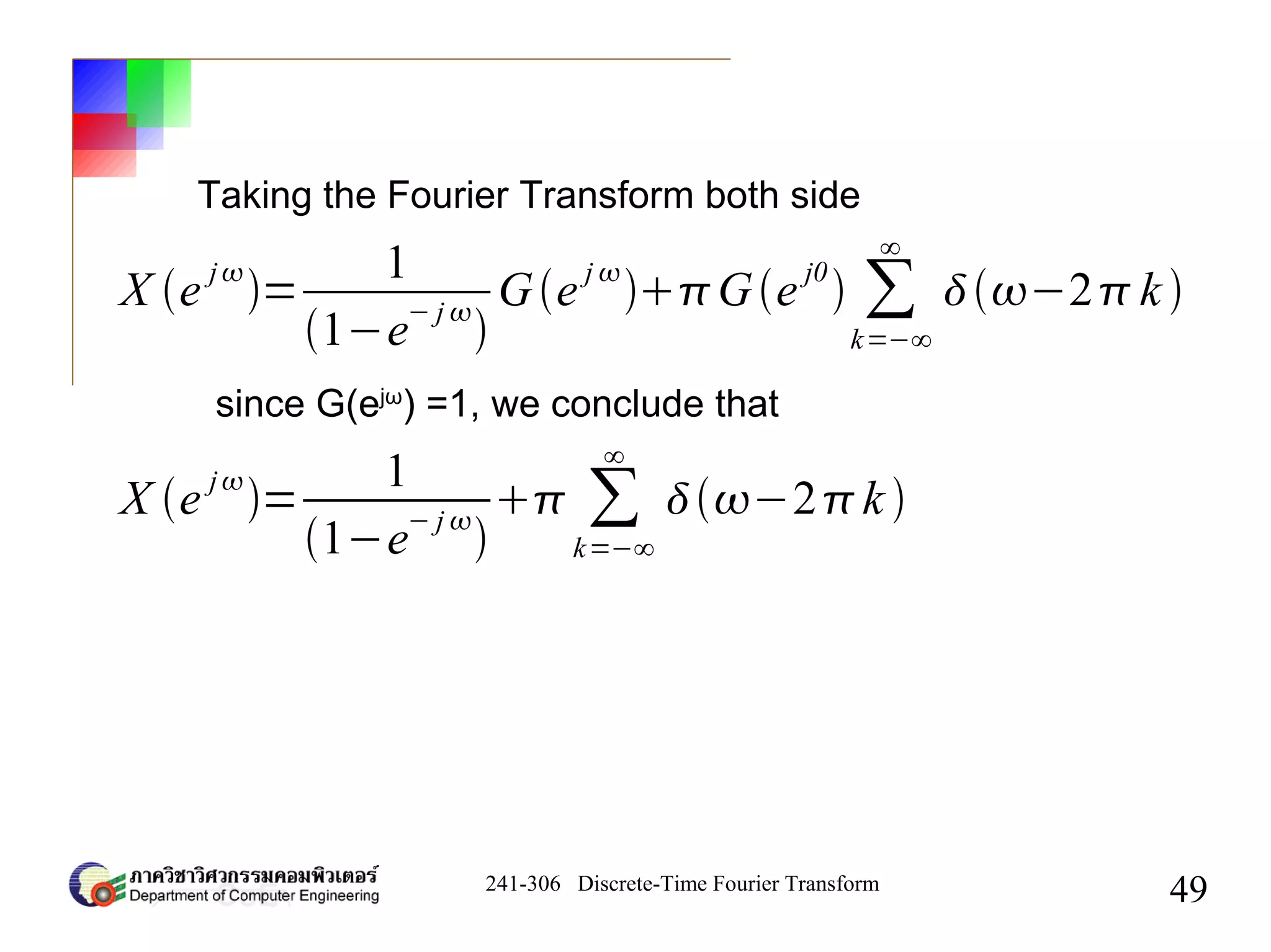
Example 5.8
g[n]=[n] ↔
F
Ge j
=1
x[n]= ∑
m=−∞
n
g[m]
Determine the Fourier transform of x[n] = u[n] by
using the accumulation property and the knowledge
that
solution
We know that](https://image.slidesharecdn.com/chapter51-200511110125/75/Chapter5-The-Discrete-Time-Fourier-Transform-48-2048.jpg)
![241-306 Discrete-Time Fourier Transform
50
Time Reversal
x[n] ↔
F
X e
j
Let
that is
x[−n] ↔
F
X e
− j
](https://image.slidesharecdn.com/chapter51-200511110125/75/Chapter5-The-Discrete-Time-Fourier-Transform-50-2048.jpg)
![241-306 Discrete-Time Fourier Transform
51
Time Expansion
xat ↔
F 1
∣a∣
X j
a
In continuous-time
Let k be a positive integer, and define the
signal
xk[n]=
{x[n/k], if n isa multipleof k
0, if n is not a multipleof k](https://image.slidesharecdn.com/chapter51-200511110125/75/Chapter5-The-Discrete-Time-Fourier-Transform-51-2048.jpg)
![241-306 Discrete-Time Fourier Transform
52
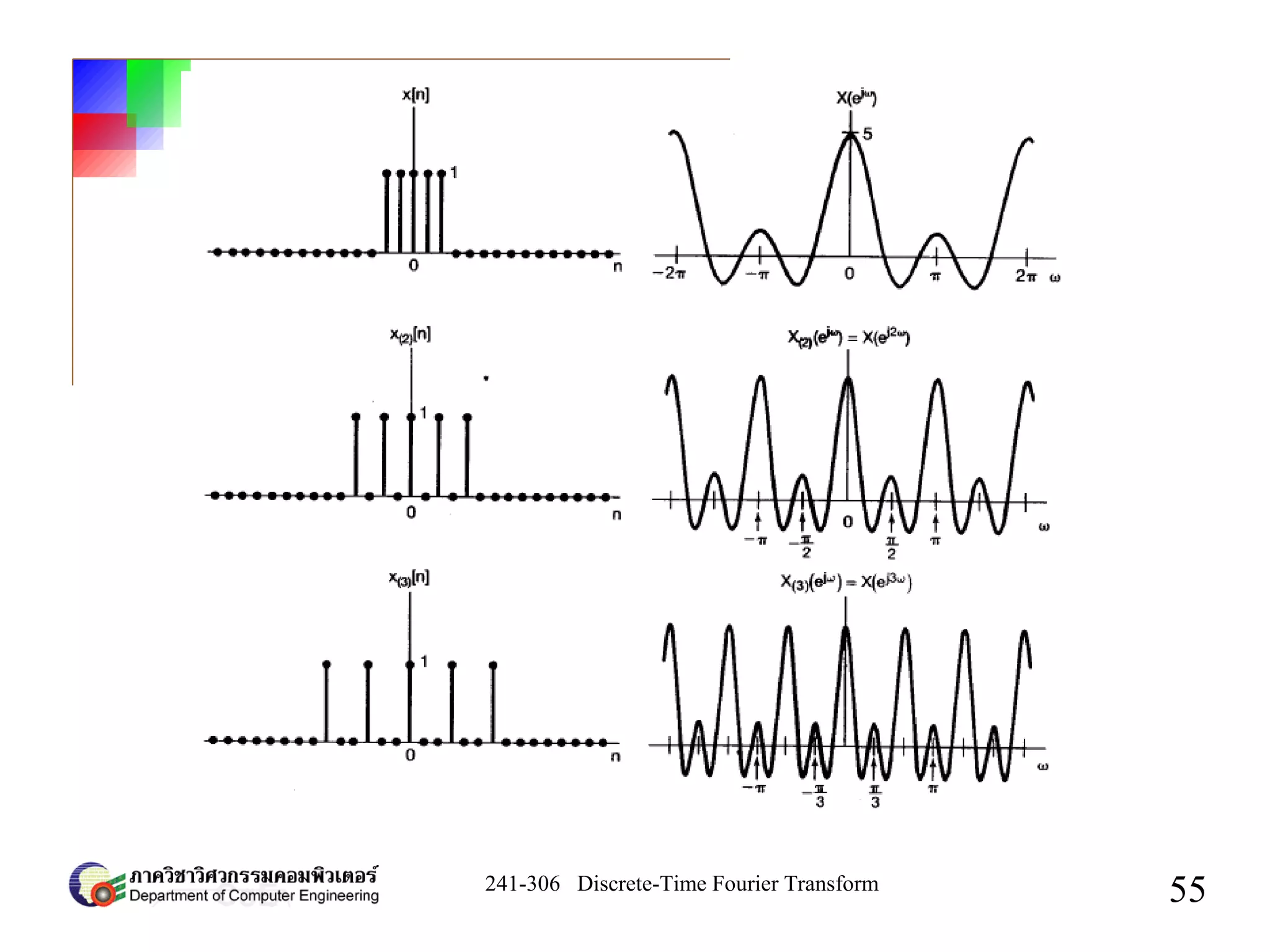
For example, k = 3, x(k)
[n] is obtained from x[n] by
placing k-1 zeros between successive values of the
original signal.](https://image.slidesharecdn.com/chapter51-200511110125/75/Chapter5-The-Discrete-Time-Fourier-Transform-52-2048.jpg)
![241-306 Discrete-Time Fourier Transform
53
We can think of x(k)
[n] as a slowed-down version
of x[n]. Since x(k)
[n] equals 0 unless n is a
multiple of k, i.e., unless n = rk, we can see that
the Fourier transform of x(k)
[n] is given by
X ke
j
= ∑
n=−∞
∞
xk[n]e
− jn
= ∑
n=−∞
∞
xk[rk]e
− j rk](https://image.slidesharecdn.com/chapter51-200511110125/75/Chapter5-The-Discrete-Time-Fourier-Transform-53-2048.jpg)
![241-306 Discrete-Time Fourier Transform
54
X ke j
= ∑
r=−∞
∞
xr[n]e− jk r
=X e jk
Since x(k)
[rk] = x[r]
That is,
xk[n] ↔
F
X e
jk
Note that as the signal is spread out and
slowed down in time by taking k>1, its Fourier
transform is compressed.](https://image.slidesharecdn.com/chapter51-200511110125/75/Chapter5-The-Discrete-Time-Fourier-Transform-54-2048.jpg)
![241-306 Discrete-Time Fourier Transform
56
Example 5.9
Determine the Fourier transform of the sequence
x[n]
x[n]= y2[n]2y2[n−1]
where](https://image.slidesharecdn.com/chapter51-200511110125/75/Chapter5-The-Discrete-Time-Fourier-Transform-56-2048.jpg)
![241-306 Discrete-Time Fourier Transform
57
solution
y2[n]=
{y[n/2], if n iseven
0 , if n isodd](https://image.slidesharecdn.com/chapter51-200511110125/75/Chapter5-The-Discrete-Time-Fourier-Transform-57-2048.jpg)
![241-306 Discrete-Time Fourier Transform
58
Y e
j
=e
− j2 sin5/2
sin/2
By using time shift property to example 5.3
and using time-expansion property,
y2[n]↔
F
e
− j4 sin5
sin](https://image.slidesharecdn.com/chapter51-200511110125/75/Chapter5-The-Discrete-Time-Fourier-Transform-58-2048.jpg)
![241-306 Discrete-Time Fourier Transform
59
2y2[n−1]↔
F
2e
− j5 sin5
sin
and using the linearity and time-shifting
properties,
Combining these two result, we have
X e
j
=e
− j4
12e
− j
sin5
sin](https://image.slidesharecdn.com/chapter51-200511110125/75/Chapter5-The-Discrete-Time-Fourier-Transform-59-2048.jpg)
![241-306 Discrete-Time Fourier Transform
60
Differentiation in frequency
x[n] ↔
F
X e
j
Let
dX e
j
d
= ∑
n=−∞
∞
− j n x[n]e
− jn
Using definition
X e
j
= ∑
n=−∞
∞
x[n]e
− jn](https://image.slidesharecdn.com/chapter51-200511110125/75/Chapter5-The-Discrete-Time-Fourier-Transform-60-2048.jpg)
![241-306 Discrete-Time Fourier Transform
61
The right hand side of this equation is the
Fourier transform of -jnx[n]. Therefore,
multiplying both sides by j, we see that
nx[n] ↔
F
j
d X e
− j
d ](https://image.slidesharecdn.com/chapter51-200511110125/75/Chapter5-The-Discrete-Time-Fourier-Transform-61-2048.jpg)
![241-306 Discrete-Time Fourier Transform
62
Parseval 's Relation
∑
n=−∞
∞
∣x[n]∣
2
=
1
2
∫
2
∣X e
j
∣
2
d
If x[n] and X(ejω
) are Fourier transform pair
Parseval's relation states that this energy can
also be determined by integrating the energy per
unit frequency, |X(ejω
)|2
/2π, over a full 2π interval
of distinct discrete-time frequencies. |X(ejω
)|2
is
referred to as the energy-density spectrum of the
signal x[n].](https://image.slidesharecdn.com/chapter51-200511110125/75/Chapter5-The-Discrete-Time-Fourier-Transform-62-2048.jpg)
![241-306 Discrete-Time Fourier Transform
63
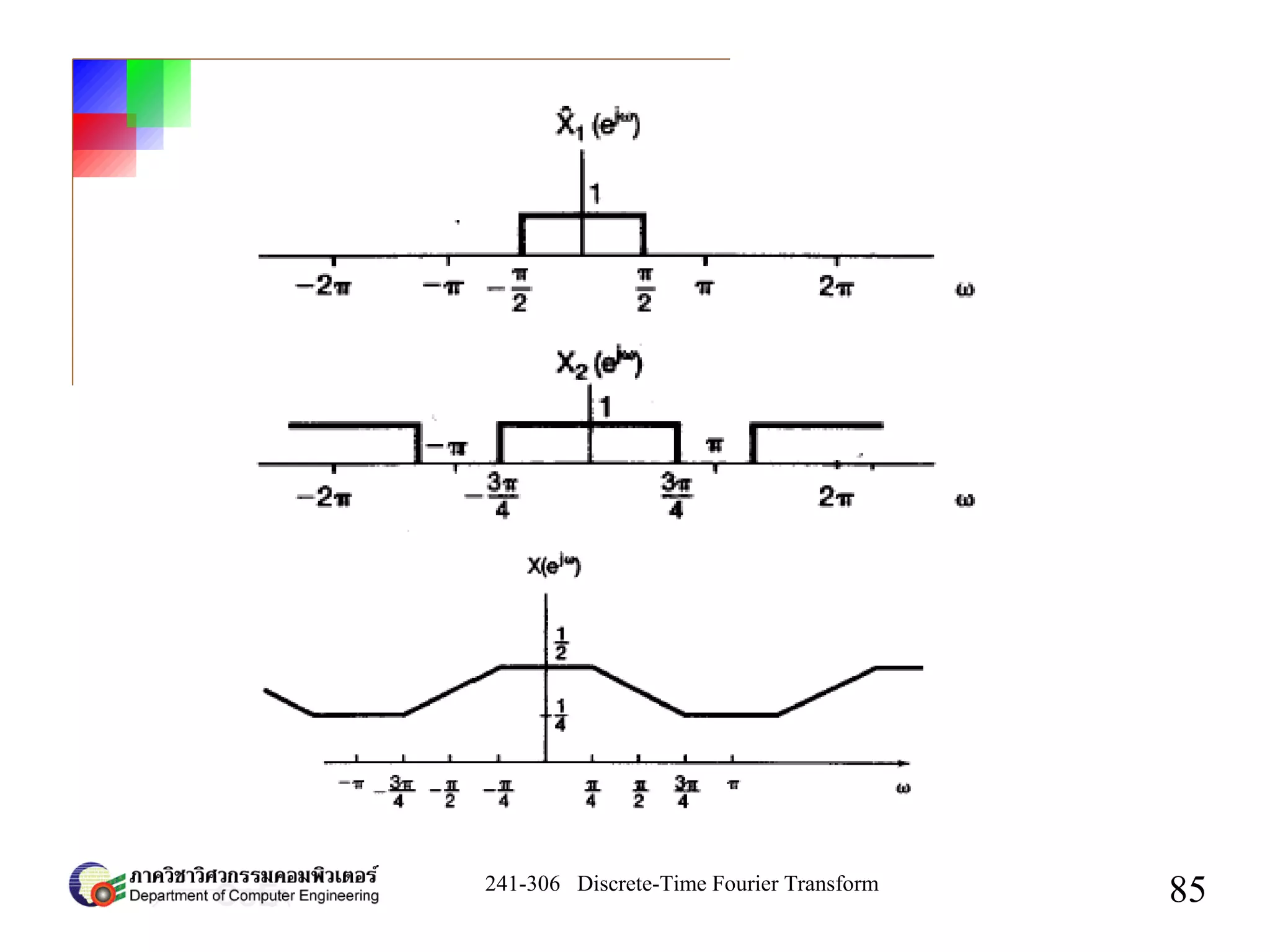
Example 4.14
Determine whether or not , in the time domain, x[n]
whose Fourier transform is depicted below, is
periodic, real, even, and/or of finite energy.](https://image.slidesharecdn.com/chapter51-200511110125/75/Chapter5-The-Discrete-Time-Fourier-Transform-63-2048.jpg)
![241-306 Discrete-Time Fourier Transform
64
solution
We note first that periodicity in the time domain
implies that the Fourier transform is zero,
expect possibly for impulses located at various
integer multiples of the fundamental frequency.
Thus is not true for X(ejω
). We conclude that
x[n] is not periodic.
From the symmetry properties for Fourier
transforms, we know that a real-valued
sequence must have a Fourier transform of
even magnitude and a phase function that is
odd. This is true for the given X(ejω
) and
∢X(ejω
). We conclude that x[n] is real.](https://image.slidesharecdn.com/chapter51-200511110125/75/Chapter5-The-Discrete-Time-Fourier-Transform-64-2048.jpg)
![241-306 Discrete-Time Fourier Transform
65
∑
n=−∞
∞
∣x[n]∣
2
dt =
1
2
∫
2
∣X e
j
∣
2
d
If x[n] is an even function, then by the
symmetry properties for real signals, X(ejω
)
must real and even but this X(ejω
) is not a real-
valued function. Consequently, x[n] is not
even.
Finally, for the finite-energy property, we may
use Parseval's relation
It clear that integrating |X(ejω
)|2
from -π to π will
yield a finite quantity. We conclude that x[n]
has finite energy.](https://image.slidesharecdn.com/chapter51-200511110125/75/Chapter5-The-Discrete-Time-Fourier-Transform-65-2048.jpg)
![241-306 Discrete-Time Fourier Transform
66
4 The Convolution Property
h[n] ↔
F
H e
j
y[n] ↔
F
Y e
j
y[n]=h[n]∗x[n] ↔
F
Y e
j
=H e
j
X e
j
If
then
x[n] ↔
F
X e
j
](https://image.slidesharecdn.com/chapter51-200511110125/75/Chapter5-The-Discrete-Time-Fourier-Transform-66-2048.jpg)
![241-306 Discrete-Time Fourier Transform
67
Example 5.11
Consider the LTI system with impulse response
h[n]=n−n0
The frequency response is
H e
j
= ∑
n=−∞
∞
[n−n0]e
− j n
=e
− jn0
For any input x[n] with Fourier transform
H(ejω
), the Fourier transform of the output is
Y ej
=e
−j n0
X e j
y[n]=xn−n0](https://image.slidesharecdn.com/chapter51-200511110125/75/Chapter5-The-Discrete-Time-Fourier-Transform-67-2048.jpg)
![241-306 Discrete-Time Fourier Transform
69
h[n]=
1
2
∫
−
H e
j
e
jn
d
=
1
2
∫
−c
e
jn
d
=
sinc n
n
solution](https://image.slidesharecdn.com/chapter51-200511110125/75/Chapter5-The-Discrete-Time-Fourier-Transform-69-2048.jpg)
![241-306 Discrete-Time Fourier Transform
70
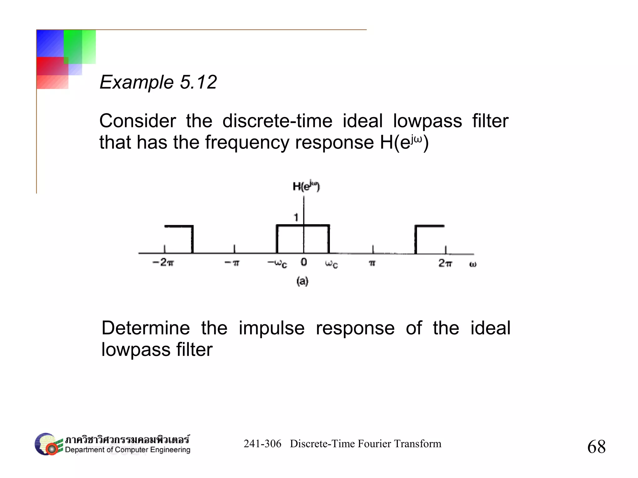
Example 5.13
Determine the frequency response of an LTI
system with impulse response
h[n]=
n
u[n], ∣∣1
to the input signal
x[n]=
n
u[n], ∣∣1](https://image.slidesharecdn.com/chapter51-200511110125/75/Chapter5-The-Discrete-Time-Fourier-Transform-70-2048.jpg)
![241-306 Discrete-Time Fourier Transform
71
solution
The Fourier transform of x[n] and h[n] are
X e
j
=
1
1−e
− j H e
j
=
1
1−e− j
Therefore
Y e j
=
1
1−e
− j
1−e
− j
](https://image.slidesharecdn.com/chapter51-200511110125/75/Chapter5-The-Discrete-Time-Fourier-Transform-71-2048.jpg)
![241-306 Discrete-Time Fourier Transform
72
Y e j
=
A
1−e− j
B
1−e− j
A=
−
, B=
−
−
y[n]=
−
n
u[n]−
−
n
u[n]
Assuming that α ≠ β, the partial fraction
expansion for Y(ejω
) takes the form
We find that
Therefore](https://image.slidesharecdn.com/chapter51-200511110125/75/Chapter5-The-Discrete-Time-Fourier-Transform-72-2048.jpg)
![241-306 Discrete-Time Fourier Transform
73
y[n]=
1
−
[n1
u[n]−n1
u[n]]
Y e
j
=
1
1−e
− j
2
1
1− e− j
2
=
j
e j d
d [ 1
1− e− j ]
or
If α = β
Recognizing this as](https://image.slidesharecdn.com/chapter51-200511110125/75/Chapter5-The-Discrete-Time-Fourier-Transform-73-2048.jpg)
![241-306 Discrete-Time Fourier Transform
74
n
u[n] ↔
F 1
1− e
− j
n
n
u[n] ↔
F
j
d
d 1
1−e
− j
We can use the dual of the differentiation
property
For the factor ejω
, we uses time-shifting property
n1
n1
u[n1] ↔
F
j e
j d
d 1
1−e
− j ](https://image.slidesharecdn.com/chapter51-200511110125/75/Chapter5-The-Discrete-Time-Fourier-Transform-74-2048.jpg)
![241-306 Discrete-Time Fourier Transform
75
Finally, accounting for the factor 1/α, we obtain
y[n]=n1
n
u[n1]
Since (n+1) is zero at n=-1
y[n]=n1
n
u[n]](https://image.slidesharecdn.com/chapter51-200511110125/75/Chapter5-The-Discrete-Time-Fourier-Transform-75-2048.jpg)
![241-306 Discrete-Time Fourier Transform
77
solution
The Fourier transform of the signal w1
[n] can be
obtain by noting that
−1n
=e
jn
so that
w1[n]=e
j n
x[n]
Using the frequency-shifting property
W1 e
j
=X e
j−
](https://image.slidesharecdn.com/chapter51-200511110125/75/Chapter5-The-Discrete-Time-Fourier-Transform-77-2048.jpg)
![241-306 Discrete-Time Fourier Transform
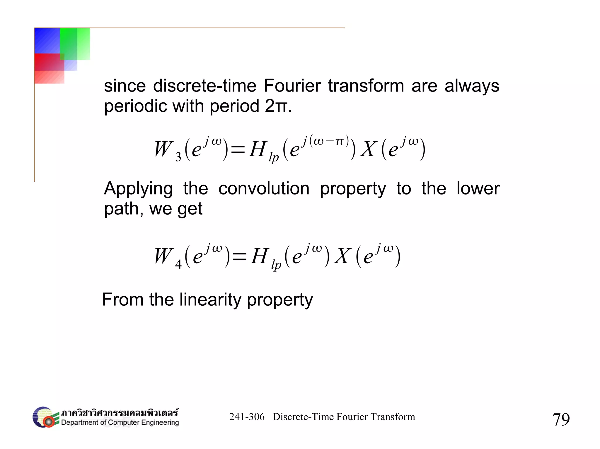
78
by convolution property
W 2e
j
=H lpe
j
X e
j−
since
w3 [n]=e jn
w2[n]
applying the frequency-shifting property
W 3e j
=W 2e j−
=H lpe
j−
X e
j−2
](https://image.slidesharecdn.com/chapter51-200511110125/75/Chapter5-The-Discrete-Time-Fourier-Transform-78-2048.jpg)
![241-306 Discrete-Time Fourier Transform
80
Y e
j
=W 3e
j
W 4e
j
=[Hlp e
j−
Hlp e
j
] X e
j
The frequency response of the overall system is
H e j
=[Hlp e j−
H lpe j
]](https://image.slidesharecdn.com/chapter51-200511110125/75/Chapter5-The-Discrete-Time-Fourier-Transform-80-2048.jpg)
![241-306 Discrete-Time Fourier Transform
81
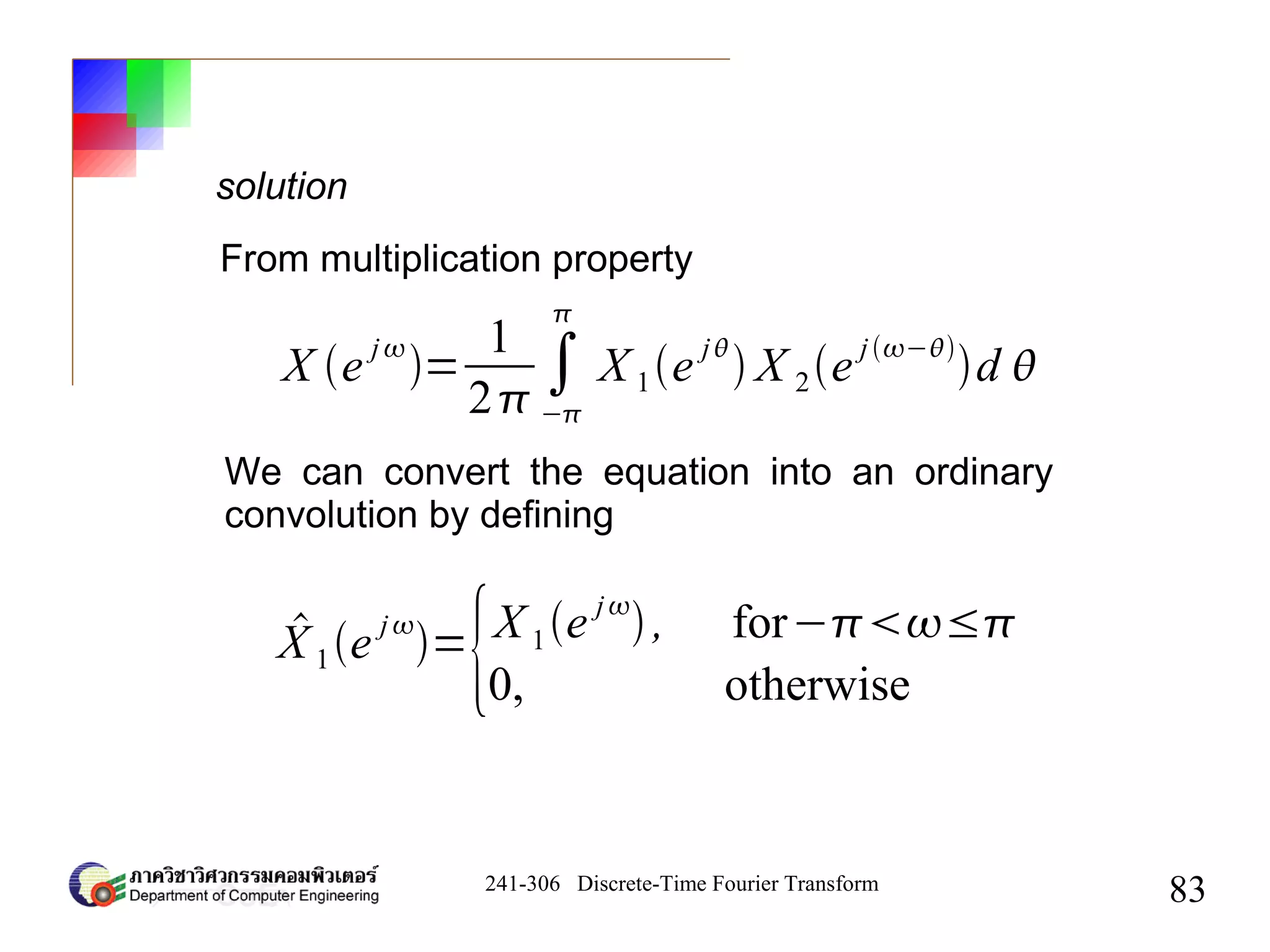
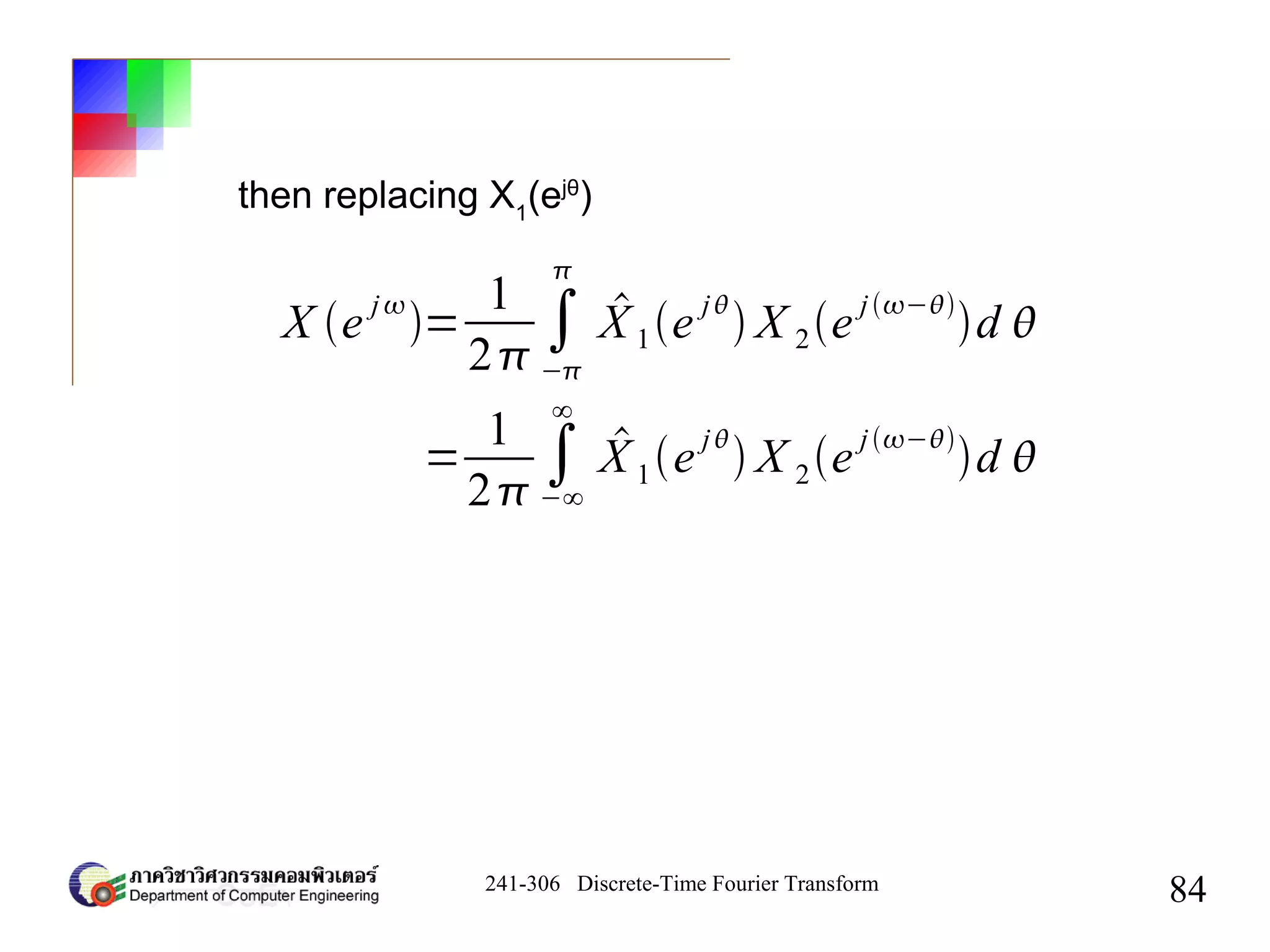
4 The Multiplication Property
y[n]=x1[n] x2[n]↔
F
R j =
1
2
∫
2
X e j
X e j−
d
The multiplication in time domain corresponds to
convolution in frequency domain
corresponds to a periodic convolution, and the
integral can be evaluated over any interval of
length 2π](https://image.slidesharecdn.com/chapter51-200511110125/75/Chapter5-The-Discrete-Time-Fourier-Transform-81-2048.jpg)
![241-306 Discrete-Time Fourier Transform
82
Example 5.15
Find the Fourier transform of the signal x[n]
x[n]=x1[n] x2[n]
where
x1[n]=
sin3n/4
n
x2[n]=
sinn/2
n](https://image.slidesharecdn.com/chapter51-200511110125/75/Chapter5-The-Discrete-Time-Fourier-Transform-82-2048.jpg)
![241-306 Discrete-Time Fourier Transform
88
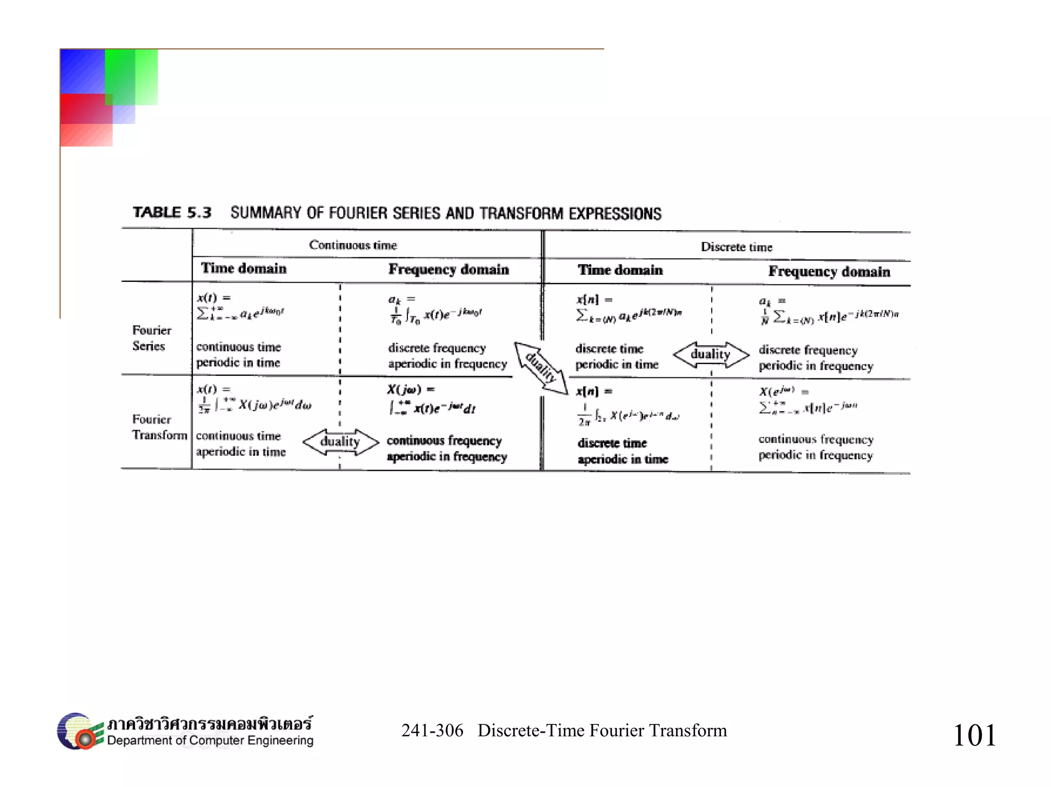
6 Duality
Duality in discrete-time Fourier Series
x[n]= ∑
k=〈 N 〉
ak e
jk 0 n
ak=
1
N
∑
n=〈N 〉
x[n]e
− jk 0 n
x[n] ↔
FS
ak
If we adopt the notation](https://image.slidesharecdn.com/chapter51-200511110125/75/Chapter5-The-Discrete-Time-Fourier-Transform-88-2048.jpg)
![241-306 Discrete-Time Fourier Transform
89
g [n]= ∑
k=〈N 〉
f [k]e
jk 0 n
f [k ]=
1
N
∑
n=〈N 〉
g [n]e
− jk 0 n
x1[n]=g[n] ↔
FS
ak= f [k ]
Suppose f[*] and g[*] are two functions such
that they are a FT pair](https://image.slidesharecdn.com/chapter51-200511110125/75/Chapter5-The-Discrete-Time-Fourier-Transform-89-2048.jpg)
![241-306 Discrete-Time Fourier Transform
90
f [n]=
1
N
∑
k=〈N 〉
g[−k]e
jk 0 n
= ∑
k=〈 N 〉
1
N
g[−k ]e
jk 0 n
then for another time-domain function such that
f [n]= ∑
k=〈N 〉
bk e
jk 0 n
x2[n]= f [n] ↔
FS
bk=
1
N
g[−k ]](https://image.slidesharecdn.com/chapter51-200511110125/75/Chapter5-The-Discrete-Time-Fourier-Transform-90-2048.jpg)
![241-306 Discrete-Time Fourier Transform
91
Example 5.16
Consider the following periodic signal with a
period of N = 9
x[n]=
{
1
9
sin5n/9
sinn/9
,n≠multiple of 9
5
9
, n=multiple of 9](https://image.slidesharecdn.com/chapter51-200511110125/75/Chapter5-The-Discrete-Time-Fourier-Transform-91-2048.jpg)
![241-306 Discrete-Time Fourier Transform
92
From chapter 3, the Fourier series coefficients for
x[n] must be in the form of a rectangular square
wave. Let g[n] be
g [n]=
{1, ∣n∣≤2
0, 2∣n∣≤4
The Fourier series coefficients bk
for g[n] can be
determined from ex. 3.12 as](https://image.slidesharecdn.com/chapter51-200511110125/75/Chapter5-The-Discrete-Time-Fourier-Transform-92-2048.jpg)
![241-306 Discrete-Time Fourier Transform
93
bk=
{
1
9
sin5k /9
sin k /9
,k≠multiple of 9
5
9
, k=multiple of 9
The Fourier series analysis equation for g[n] is
bk=
1
9
∑
n=−2
2
1e
− j 2nk /9](https://image.slidesharecdn.com/chapter51-200511110125/75/Chapter5-The-Discrete-Time-Fourier-Transform-93-2048.jpg)
![241-306 Discrete-Time Fourier Transform
94
x[n]=
1
9
∑
k=−2
2
1e
− j 2n k/9
Let k' = -k
x[n]=
1
9
∑
k '=−2
2
1e
j 2n k ' /9
Interchanging the names of the variables k and n
and noting that x[n] = bn
, we find that](https://image.slidesharecdn.com/chapter51-200511110125/75/Chapter5-The-Discrete-Time-Fourier-Transform-94-2048.jpg)
![241-306 Discrete-Time Fourier Transform
95
Finally, moving the factor 1/9 inside the
summation, we see that the right side of this
equation has the form of the synthesis equation
for x[n]. We conclude that the FS coefficients are
ak=
{1, ∣k∣≤2
0, 2∣k∣≤4](https://image.slidesharecdn.com/chapter51-200511110125/75/Chapter5-The-Discrete-Time-Fourier-Transform-95-2048.jpg)
![241-306 Discrete-Time Fourier Transform
96
x[n]=
1
2
∫
2
X e
j
e
jn
d
X e
j
= ∑
n=−∞
∞
x[n]e
jn
xt= ∑
k=−∞
∞
ak e
j k 0 t
ak=
1
T
∫
T
xte
− j k 0t
d t
Duality between the discrete-time Fourier transform
and the continuous-time Fourier series
DTFT
CTFS](https://image.slidesharecdn.com/chapter51-200511110125/75/Chapter5-The-Discrete-Time-Fourier-Transform-96-2048.jpg)
![241-306 Discrete-Time Fourier Transform
97
Example 5.17
Determine the discrete-time Fourier transform
of the sequence
x[n]=
sin n/2
n](https://image.slidesharecdn.com/chapter51-200511110125/75/Chapter5-The-Discrete-Time-Fourier-Transform-97-2048.jpg)
![241-306 Discrete-Time Fourier Transform
98
g t=
{1, ∣t∣≤T1
0, T1∣t∣≤
To use duality, we first must identify a
continuous-time signal g(t) with period T= 2π and
Fourier coefficients ak
= x[k]. From Ex. 3.5, we
know that if g(t) is periodic and with
then
ak=
sink T1
k
Solution](https://image.slidesharecdn.com/chapter51-200511110125/75/Chapter5-The-Discrete-Time-Fourier-Transform-98-2048.jpg)
![241-306 Discrete-Time Fourier Transform
99
Consequently, if we take T1
= π/2, we will have
ak
=x[k]
sink /2
k
=
1
2
∫
−
g te
− j k t
dt
=
1
2
∫
−/2
/2
1e
− j k t
dt
Rename k as n and t as ω, we have
sin n/2
n
=
1
2
∫
−/2
/2
1e
− j n
d ](https://image.slidesharecdn.com/chapter51-200511110125/75/Chapter5-The-Discrete-Time-Fourier-Transform-99-2048.jpg)
![241-306 Discrete-Time Fourier Transform
100
Replacing n by -n
sin n/2
n
=
1
2
∫
−/2
/2
1e j n
d
On the right hand side has the form of the
x[n]=
1
2
∫
2
X e j
e jn
d
where
X e
j
=
{1, ∣∣≤/2
0, /2∣∣≤](https://image.slidesharecdn.com/chapter51-200511110125/75/Chapter5-The-Discrete-Time-Fourier-Transform-100-2048.jpg)
![241-306 Discrete-Time Fourier Transform
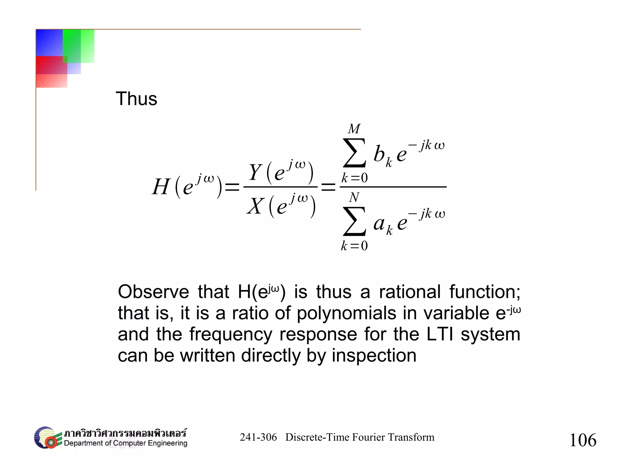
102
7 Systems Characterized by Linear Constant-
Coefficient Difference Equations
A linear constant-coefficient differential equation
with input x[n] and output y[n] is of the form
∑
k=0
N
ak y[n−k ]=∑
k=0
M
bk x[n−k ]](https://image.slidesharecdn.com/chapter51-200511110125/75/Chapter5-The-Discrete-Time-Fourier-Transform-102-2048.jpg)
![241-306 Discrete-Time Fourier Transform
103
Y e
j
=H e
j
X e
j
H e
j
=
Y e
j
X e
j
By the convolution property
or
where X(ejω
), Y(ejω
) and H(ejω
) are the Fourier
transforms of the input x[n], output y[n] and
impulse response h[n].](https://image.slidesharecdn.com/chapter51-200511110125/75/Chapter5-The-Discrete-Time-Fourier-Transform-103-2048.jpg)
![241-306 Discrete-Time Fourier Transform
104
F
{∑
k=0
N
ak y[n−k ]
}=F
{∑
k=0
M
bk x[n−k ]
}
∑
k=0
N
ak F {y[n−k ]}=∑
k=0
M
bk F {x[n−k ]}
consider applying the Fourier transform to the
equation in slide before
from linear property](https://image.slidesharecdn.com/chapter51-200511110125/75/Chapter5-The-Discrete-Time-Fourier-Transform-104-2048.jpg)
![241-306 Discrete-Time Fourier Transform
105
Y e j
[∑
k=0
N
ak e− j k
]=X e j
[∑
k=0
M
bk e− j k
]
∑
k=0
N
ak e
− j
k
Y e
j
=∑
k=0
M
bk e
− j
k
X e
j
and from the differentiation property
or](https://image.slidesharecdn.com/chapter51-200511110125/75/Chapter5-The-Discrete-Time-Fourier-Transform-105-2048.jpg)
![241-306 Discrete-Time Fourier Transform
107
Example 5.18
Find the impulse response of the LTI system
y[n]−a y[n−1]=x[n]
with |a| > 1
Solution
Fourier transform of the system is
Y e j
−ae− j
Y e j
=X e j
](https://image.slidesharecdn.com/chapter51-200511110125/75/Chapter5-The-Discrete-Time-Fourier-Transform-107-2048.jpg)
![241-306 Discrete-Time Fourier Transform
108
1−ae
− j
Y e
j
=X e
j
H e
j
=
Y e
j
X e
j
=
1
1−ae
− j
From Example 5.1, the inverse Fourier
Transform of equation above is
h[n]=a
n
u[n]](https://image.slidesharecdn.com/chapter51-200511110125/75/Chapter5-The-Discrete-Time-Fourier-Transform-108-2048.jpg)
![241-306 Discrete-Time Fourier Transform
109
Example 5.19
Find the impulse response of the LTI system
y[n]−
3
4
y[n−1]
1
8
y[n−2]=2x[n]
Solution
The frequency response is
H e
j
=
2
1−
3
4
e
− j
1
8
e
− j 2](https://image.slidesharecdn.com/chapter51-200511110125/75/Chapter5-The-Discrete-Time-Fourier-Transform-109-2048.jpg)
![241-306 Discrete-Time Fourier Transform
110
We factor the denominator of the right-hand side
By using the partial-fraction expansion
The inverse Fourier transform of each term
h[n]=41
2
n
u[n]−21
4
n
u[n]
H e
j
=
2
1−
1
2
e
− j
1−
1
4
e
− j
H e j
=
4
1−
1
2
e− j
−
2
1−
1
4
e− j](https://image.slidesharecdn.com/chapter51-200511110125/75/Chapter5-The-Discrete-Time-Fourier-Transform-110-2048.jpg)
![241-306 Discrete-Time Fourier Transform
111
Example 5.20
Consider the system of Example 5.19, find the
output of the system when the input is
x[n]=1
4
n
u[n]
Solution
Y e
j
=H e
j
X e
j
=
[
2
1−
1
2
e
− j
1−
1
4
e
− j
][
1
1−
1
4
e
− j
]](https://image.slidesharecdn.com/chapter51-200511110125/75/Chapter5-The-Discrete-Time-Fourier-Transform-111-2048.jpg)
![241-306 Discrete-Time Fourier Transform
112
By using the partial-fraction expansion
Y e
j
=
B11
1−
1
4
e
− j
B12
1−
1
4
e
− j
2
B21
1−
1
2
e
− j
Y e
j
=
[
2
1−
1
2
e
− j
1−
1
4
e
− j
2
]
=−
4
1−
1
4
e
− j
−
2
1−
1
4
e
− j
2
8
1−
1
2
e
− j ](https://image.slidesharecdn.com/chapter51-200511110125/75/Chapter5-The-Discrete-Time-Fourier-Transform-112-2048.jpg)
![241-306 Discrete-Time Fourier Transform
113
The inverse Fourier transform of each term
y[n]=
{−41
4
n
−2n11
4
n
81
2
n
}u[n]](https://image.slidesharecdn.com/chapter51-200511110125/75/Chapter5-The-Discrete-Time-Fourier-Transform-113-2048.jpg)

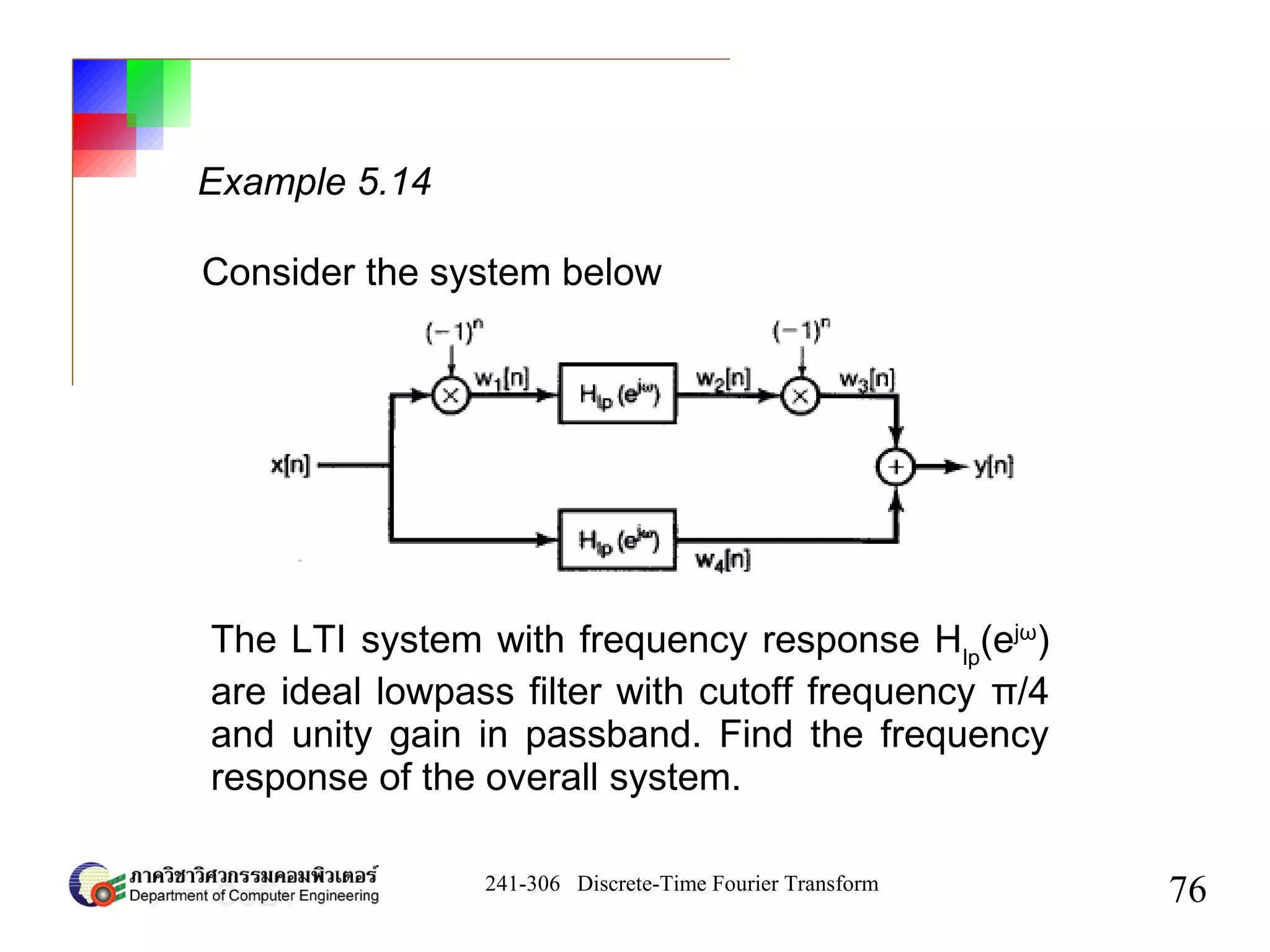
This document discusses the discrete-time Fourier transform (DTFT). It begins by introducing the DTFT and how it can be used to represent aperiodic signals as the sum of complex exponentials. Several properties of the DTFT are then discussed, including linearity, time/frequency shifting, periodicity, and conjugate symmetry. Examples are provided to illustrate how to compute the DTFT of simple signals. The document also discusses how the DTFT can be used to represent periodic signals and impulse trains.
Introduction to DTFT and its significance. Overview of topics including representation, properties, and systems characterized by linear constant-coefficient difference equations.
Details on representing aperiodic signals using DTFT. Defines formula for periodic sequences and inverses, highlighting key equations and properties.
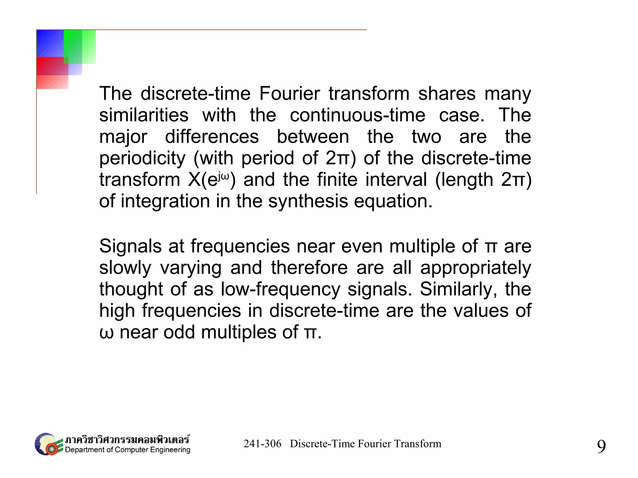
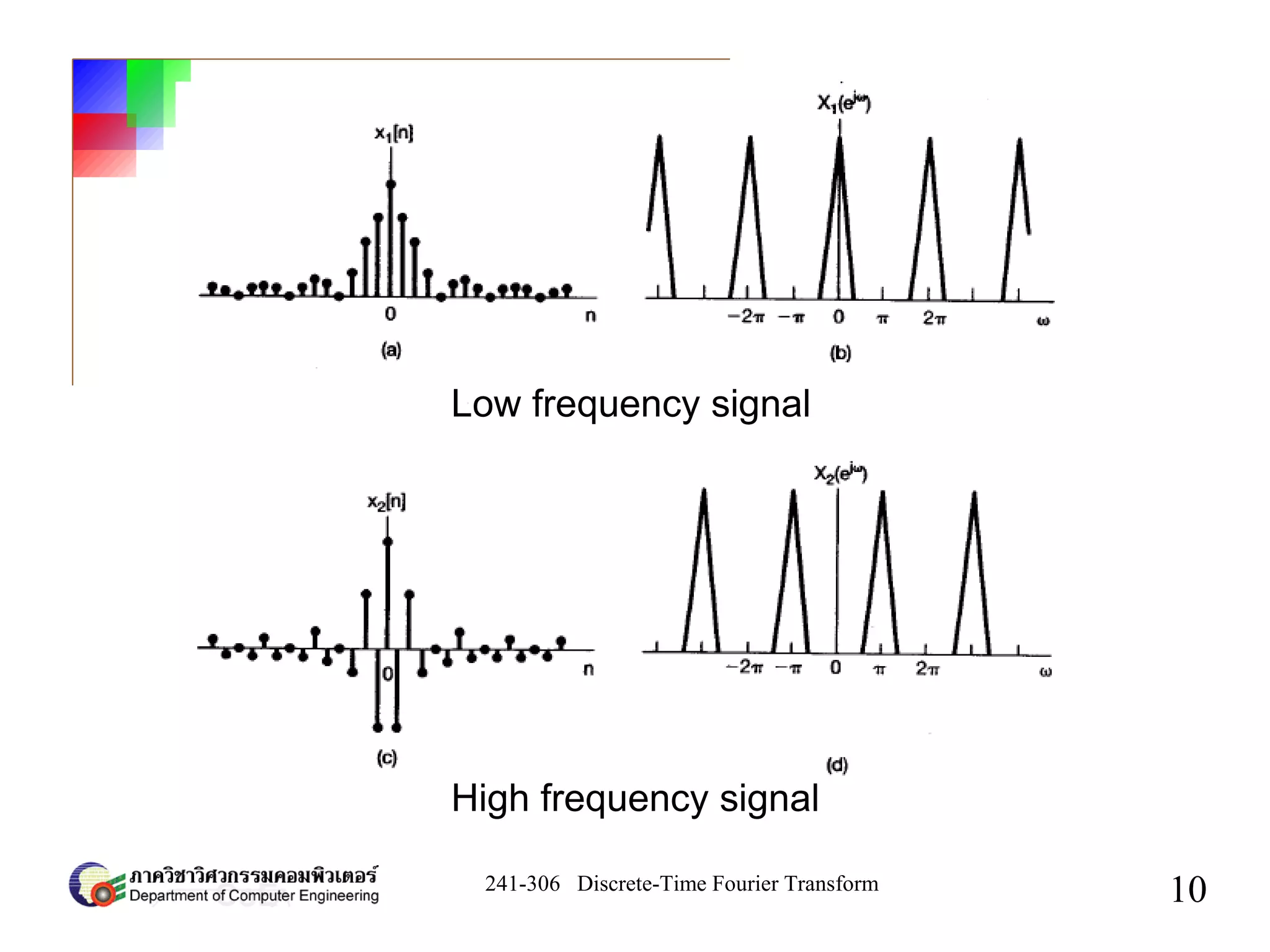
Discussions on periodicity and frequency characteristics of DTFT. Examples illustrate low and high frequency behavior.
Examples of DTFT applications for specific signals, including transformations and associated solutions.
Conditions for the convergence of Fourier transforms, demonstrating synthesis equations and approximations for aperiodic signals.
Explains Fourier Transform for periodic signals, discusses examples and visualizes impulse train transforms.
Key properties including periodicity, linearity, time shifting, and frequency shifting, with examples demonstrating their applications.
Demonstrates properties related to differentiating and accumulating sequences, with relevant examples illustrating calculations.
Discusses systems defined by difference equations, illustrating the relationship between input/output and the corresponding Fourier transforms.


![Digital Signal Processing[ECEG-3171]-Ch1_L03](https://cdn.slidesharecdn.com/ss_thumbnails/dspl3-180427094423-thumbnail.jpg?width=640&height=640&fit=bounds)