Fourier transforms & fft algorithm (paul heckbert, 1998) by tantanoid
This document provides an overview of Fourier transforms and the fast Fourier transform (FFT) algorithm. It defines the continuous and discrete Fourier transforms, discusses their properties and examples. The FFT is introduced as an efficient algorithm for computing the discrete Fourier transform (DFT) in O(N log N) time rather than O(N2) time. The FFT decomposes the DFT calculation into butterfly operations between stages for inputs in bit-reversed order.
Fourier transforms & fft algorithm (paul heckbert, 1998) by tantanoid
1.
Notes 3, ComputerGraphics 2, 15-463
Fourier Transforms and the
Fast Fourier Transform (FFT) Algorithm
Paul Heckbert
Feb. 1995
Revised 27 Jan. 1998
We start in the continuous world; then we get discrete.
Definition of the Fourier Transform
The Fourier transform (FT) of the function f (x) is the function F(ω), where:
F(ω) =
∞
−∞
f (x)e−iωx
dx
and the inverse Fourier transform is
f (x) =
1
2π
∞
−∞
F(ω)eiωx
dω
Recall that i =
√
−1 and eiθ
= cos θ + i sinθ.
Think of it as a transformation into a different set of basis functions. The Fourier trans-
form uses complex exponentials (sinusoids) of various frequencies as its basis functions.
(Other transforms, such as Z, Laplace, Cosine, Wavelet, and Hartley, use different basis
functions).
A Fourier transform pair is often written f (x) ↔ F(ω), or F ( f (x)) = F(ω) where F
is the Fourier transform operator.
If f (x) is thought of as a signal (i.e. input data) then we call F(ω) the signal’s spectrum.
If f is thought of as the impulse response of a filter (which operates on input data to produce
output data) then we call F the filter’s frequency response. (Occasionally the line between
what’s signal and what’s filter becomes blurry).
1
2.
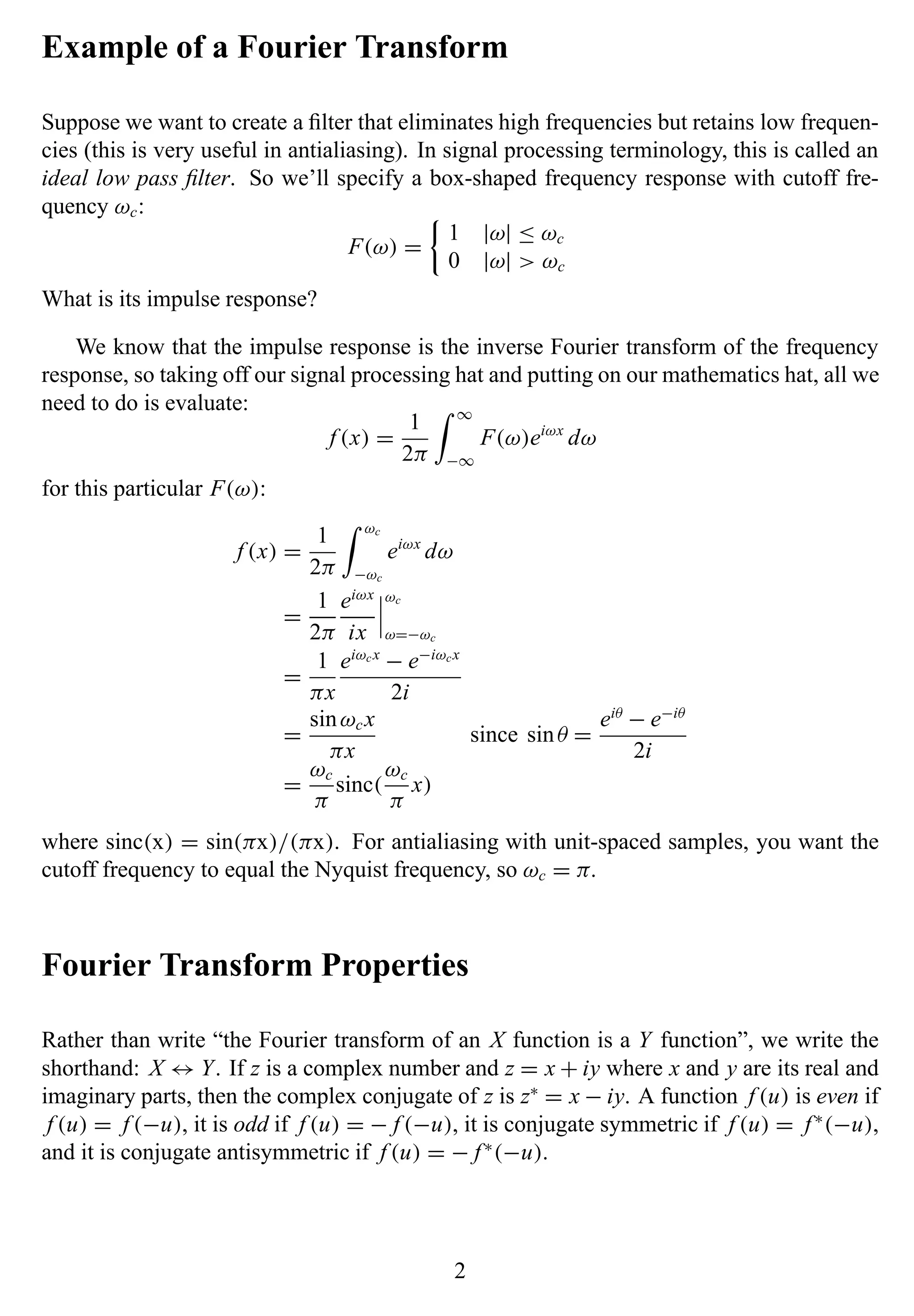
Example of aFourier Transform
Suppose we want to create a filter that eliminates high frequencies but retains low frequen-
cies (this is very useful in antialiasing). In signal processing terminology, this is called an
ideal low pass filter. So we’ll specify a box-shaped frequency response with cutoff fre-
quency ωc:
F(ω) =
1 |ω| ≤ ωc
0 |ω| > ωc
What is its impulse response?
We know that the impulse response is the inverse Fourier transform of the frequency
response, so taking off our signal processing hat and putting on our mathematics hat, all we
need to do is evaluate:
f (x) =
1
2π
∞
−∞
F(ω)eiωx
dω
for this particular F(ω):
f (x) =
1
2π
ωc
−ωc
eiωx
dω
=
1
2π
eiωx
ix
ωc
ω=−ωc
=
1
πx
eiωcx
− e−iωcx
2i
=
sinωcx
πx
since sinθ =
eiθ
− e−iθ
2i
=
ωc
π
sinc(
ωc
π
x)
where sinc(x) = sin(πx)/(πx). For antialiasing with unit-spaced samples, you want the
cutoff frequency to equal the Nyquist frequency, so ωc = π.
Fourier Transform Properties
Rather than write “the Fourier transform of an X function is a Y function”, we write the
shorthand: X ↔ Y. If z is a complex number and z = x + iy where x and y are its real and
imaginary parts, then the complex conjugate of z is z∗
= x − iy. A function f (u) is even if
f (u) = f (−u), it is odd if f (u) = − f (−u), it is conjugate symmetric if f (u) = f ∗
(−u),
and it is conjugate antisymmetric if f (u) = − f ∗
(−u).
2
3.
discrete ↔ periodic
periodic↔ discrete
discrete, periodic ↔ discrete, periodic
real ↔ conjugate symmetric
imaginary ↔ conjugate antisymmetric
box ↔ sinc
sinc ↔ box
Gaussian ↔ Gaussian
impulse ↔ constant
impulse train ↔ impulse train
(can you prove the above?)
When a signal is scaled up spatially, its spectrum is scaled down in frequency, and vice
versa: f (ax) ↔ F(ω/a) for any real, nonzero a.
Convolution Theorem
The Fourier transform of a convolution of two signals is the product of their Fourier trans-
forms: f ∗ g ↔ FG. The convolution of two continuous signals f and g is
( f ∗ g)(x) =
+∞
−∞
f (t)g(x − t)dt
So
+∞
−∞
f (t)g(x − t)dt ↔ F(ω)G(ω).
The Fourier transform of a product of two signals is the convolution of their Fourier
transforms: fg ↔ F ∗ G/2π.
Delta Functions
The (Dirac) delta function δ(x) is defined such that δ(x) = 0 for all x = 0,
+∞
−∞
δ(t)dt = 1,
and for any f (x):
( f ∗ δ)(x) =
+∞
−∞
f (t)δ(x − t)dt = f (x)
The latter is called the sifting property of delta functions. Because convolution with a delta
is linear shift-invariant filtering, translating the delta by a will translate the output by a:
f (x) ∗ δ(x − a) (x) = f (x − a)
3
4.
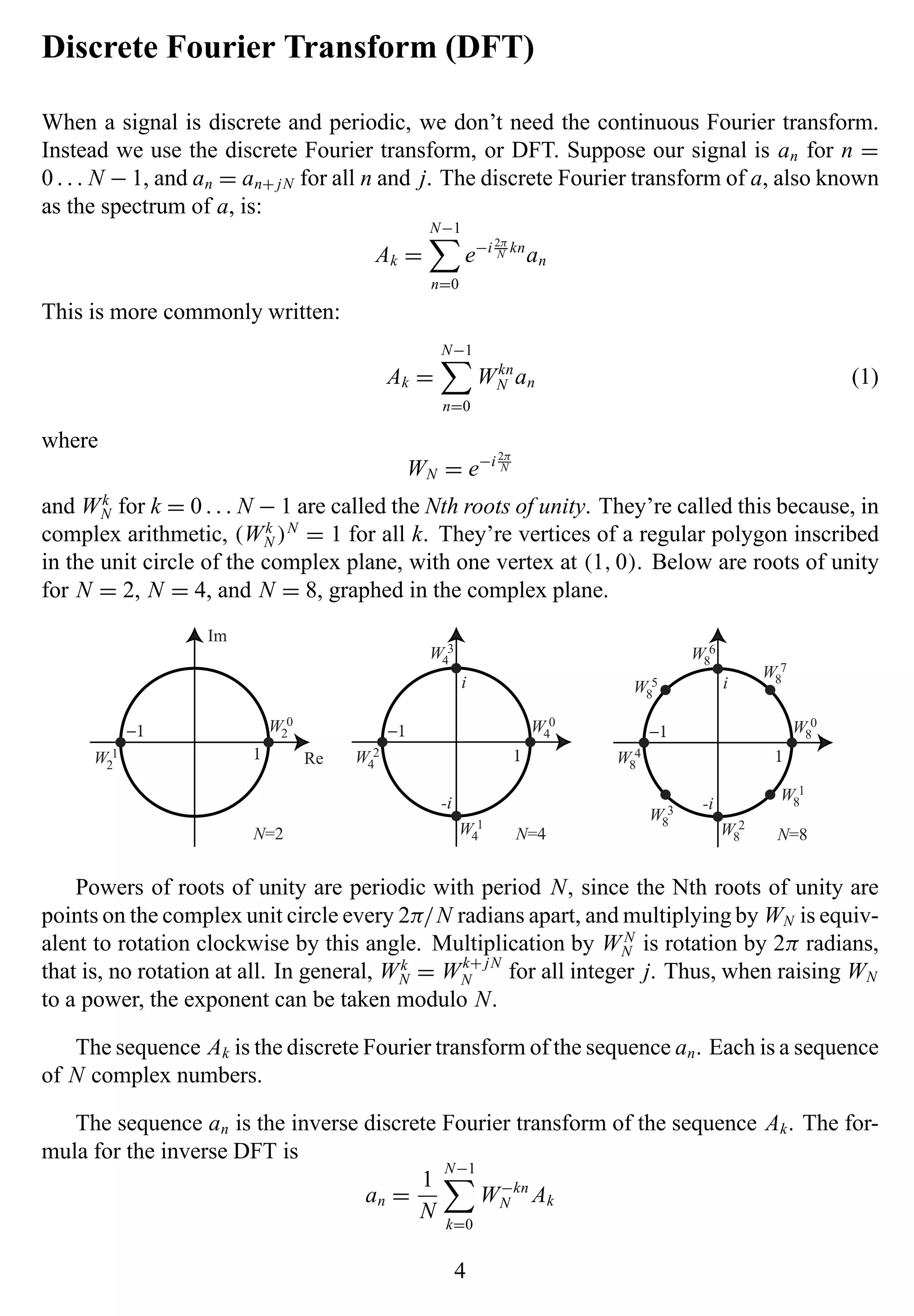
Discrete Fourier Transform(DFT)
When a signal is discrete and periodic, we don’t need the continuous Fourier transform.
Instead we use the discrete Fourier transform, or DFT. Suppose our signal is an for n =
0. . . N − 1, and an = an+ jN for all n and j. The discrete Fourier transform of a, also known
as the spectrum of a, is:
Ak =
N−1
n=0
e−i 2π
N kn
an
This is more commonly written:
Ak =
N−1
n=0
Wkn
N an (1)
where
WN = e−i 2π
N
and Wk
N for k = 0. . . N − 1 are called the Nth roots of unity. They’re called this because, in
complex arithmetic, (Wk
N )N
= 1 for all k. They’re vertices of a regular polygon inscribed
in the unit circle of the complex plane, with one vertex at (1,0). Below are roots of unity
for N = 2, N = 4, and N = 8, graphed in the complex plane.
W4
2
Re
Im
N=2
W2
0
W2
1
N=4
W4
0
W4
3
W4
1
1
−1 −1
1
i
-i
W8
4
N=8
W8
0
W8
6
W8
2
−1
1
i
-i
W8
7
W8
5
W8
3
W8
1
Powers of roots of unity are periodic with period N, since the Nth roots of unity are
points on the complex unit circle every 2π/N radians apart, and multiplying by WN is equiv-
alent to rotation clockwise by this angle. Multiplication by WN
N is rotation by 2π radians,
that is, no rotation at all. In general, Wk
N = Wk+ jN
N for all integer j. Thus, when raising WN
to a power, the exponent can be taken modulo N.
The sequence Ak is the discrete Fourier transform of the sequence an. Each is a sequence
of N complex numbers.
The sequence an is the inverse discrete Fourier transform of the sequence Ak. The for-
mula for the inverse DFT is
an =
1
N
N−1
k=0
W−kn
N Ak
4
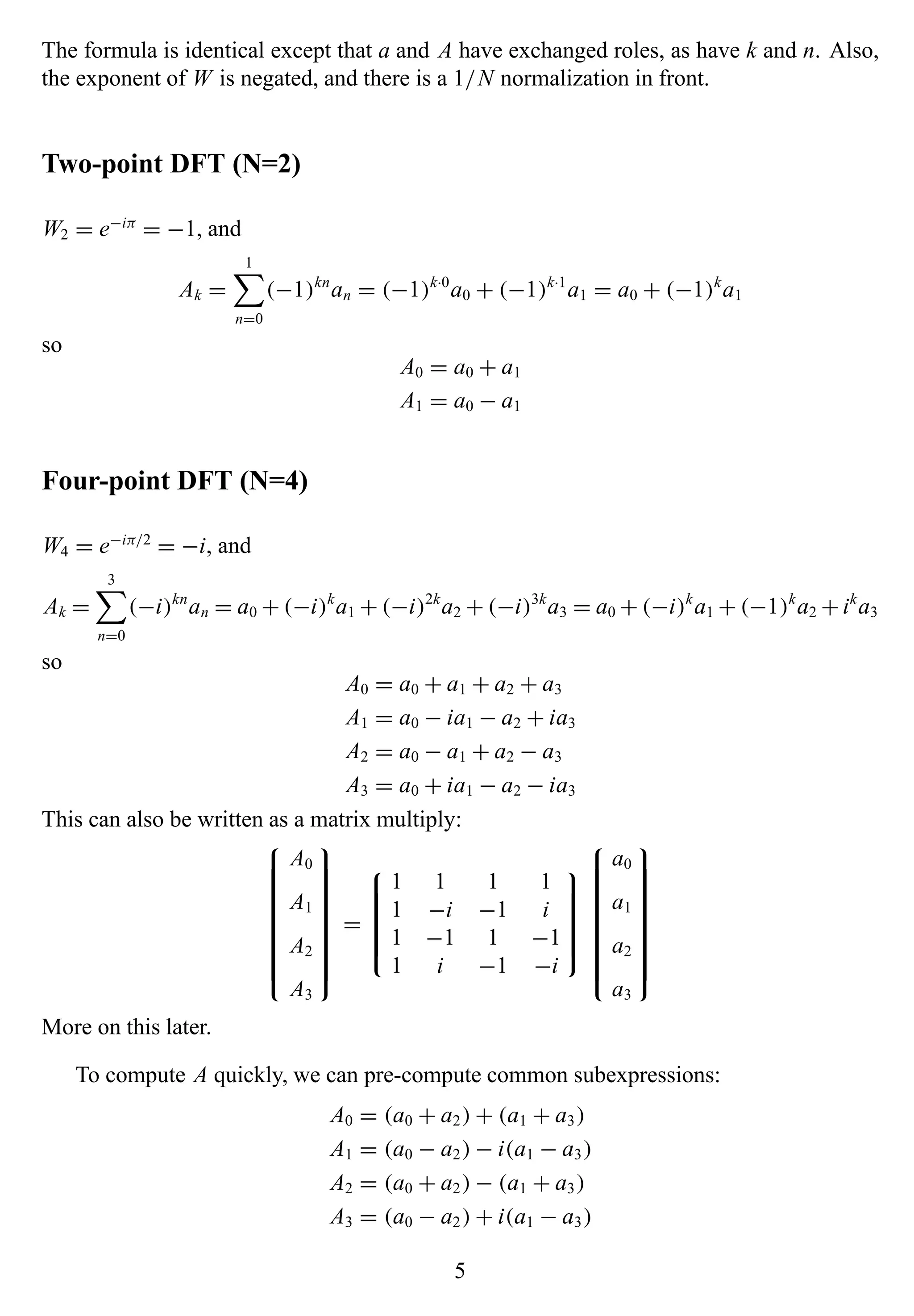
5.
The formula isidentical except that a and A have exchanged roles, as have k and n. Also,
the exponent of W is negated, and there is a 1/N normalization in front.
Two-point DFT (N=2)
W2 = e−iπ
= −1, and
Ak =
1
n=0
(−1)kn
an = (−1)k·0
a0 + (−1)k·1
a1 = a0 + (−1)k
a1
so
A0 = a0 + a1
A1 = a0 − a1
Four-point DFT (N=4)
W4 = e−iπ/2
= −i, and
Ak =
3
n=0
(−i)kn
an = a0 + (−i)k
a1 + (−i)2k
a2 + (−i)3k
a3 = a0 + (−i)k
a1 + (−1)k
a2 +ik
a3
so
A0 = a0 + a1 + a2 + a3
A1 = a0 − ia1 − a2 + ia3
A2 = a0 − a1 + a2 − a3
A3 = a0 + ia1 − a2 − ia3
This can also be written as a matrix multiply:
A0
A1
A2
A3
=
1 1 1 1
1 −i −1 i
1 −1 1 −1
1 i −1 −i
a0
a1
a2
a3
More on this later.
To compute A quickly, we can pre-compute common subexpressions:
A0 = (a0 + a2) + (a1 + a3)
A1 = (a0 − a2) − i(a1 − a3)
A2 = (a0 + a2) − (a1 + a3)
A3 = (a0 − a2) + i(a1 − a3)
5
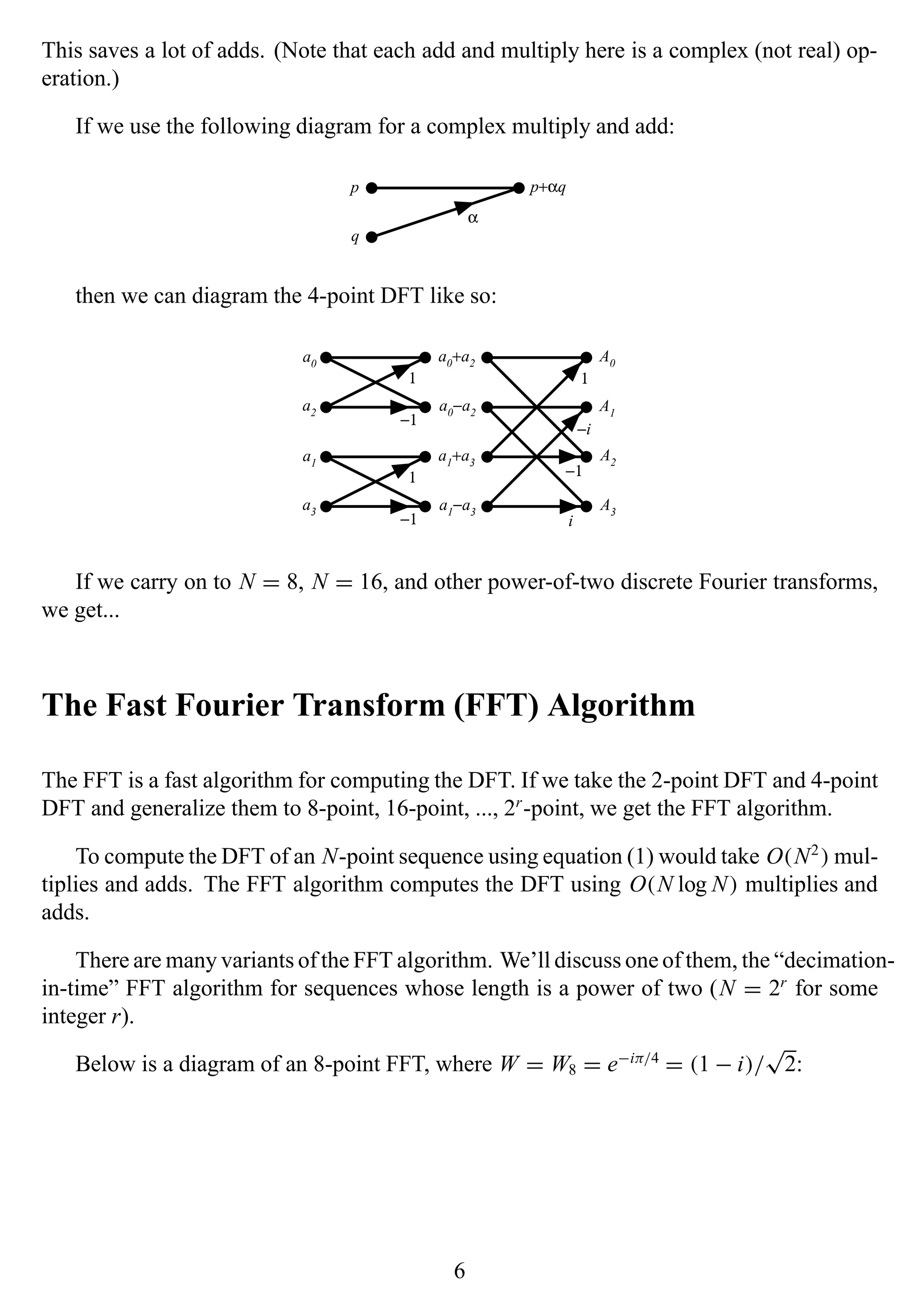
6.
This saves alot of adds. (Note that each add and multiply here is a complex (not real) op-
eration.)
If we use the following diagram for a complex multiply and add:
p
q
α
p+αq
then we can diagram the 4-point DFT like so:
a0
1
a0+a2
a2
−1
a0−a2
a1
1
a1
+a3
a3
−1
a1
−a3
1
A0
−1
A2
−i
A1
i
A3
If we carry on to N = 8, N = 16, and other power-of-two discrete Fourier transforms,
we get...
The Fast Fourier Transform (FFT) Algorithm
The FFT is a fast algorithm for computing the DFT. If we take the 2-point DFT and 4-point
DFT and generalize them to 8-point, 16-point, ..., 2r
-point, we get the FFT algorithm.
To compute the DFT of an N-point sequence using equation (1) would take O(N2
) mul-
tiplies and adds. The FFT algorithm computes the DFT using O(N log N) multiplies and
adds.
There are many variants of the FFT algorithm. We’ll discuss one of them, the “decimation-
in-time” FFT algorithm for sequences whose length is a power of two (N = 2r
for some
integer r).
Below is a diagram of an 8-point FFT, where W = W8 = e−iπ/4
= (1 − i)/
√
2:
6
7.
a0
1
a4
−1
a2
1
a6
−1
W 0
A0
W 2
W4
W 6
a1
1
a5
−1
a3
1
a7
−1
W 0
W 2
W 4
W 6
W 0
W 4
W 1
W 5
W 2
W 6
W 3
W 7
A1
A2
A3
A4
A5
A6
A7
Butterflies and Bit-Reversal. The FFT algorithm decomposes the DFT into log2 N stages,
each of which consists of N/2 butterfly computations. Each butterfly takes two complex
numbers p and q and computes from them two other numbers, p + αq and p − αq, where
α is a complex number. Below is a diagram of a butterfly operation.
p
α
p+αq
q
−α
p−αq
In the diagram of the 8-point FFT above, note that the inputs aren’t in normal order:
a0, a1, a2, a3, a4, a5, a6, a7, they’re in the bizarre order: a0, a4, a2, a6, a1, a5, a3, a7. Why
this sequence?
Below is a table of j and the index of the jth input sample, nj:
j 0 1 2 3 4 5 6 7
nj 0 4 2 6 1 5 3 7
j base 2 000 001 010 011 100 101 110 111
nj base 2 000 100 010 110 001 101 011 111
The pattern is obvious if j and nj are written in binary (last two rows of the table). Observe
that each nj is the bit-reversal of j. The sequence is also related to breadth-first traversal of
a binary tree.
It turns out that this FFT algorithm is simplest if the input array is rearranged to be in
bit-reversed order. The re-ordering can be done in one pass through the array a:
7
8.
for j =0 to N-1
nj = bit_reverse(j)
if (j<nj) swap a[j] and a[nj]
General FFT and IFFT Algorithm for N = 2r
. The previously diagrammed algorithm
for the 8-point FFT is easily generalized to any power of two. The input array is bit-reversed,
and the butterfly coefficients can be seen to have exponents in arithmetic sequence modulo
N. For example, for N = 8, the butterfly coefficients on the last stage in the diagram are
W0
, W1
, W2
, W3
, W4
, W5
, W6
, W7
. That is, powers of W in sequence. The coefficients
in the previous stage have exponents 0,2,4,6,0,2,4,6, which is equivalent to the sequence
0,2,4,6,8,10,12,14 modulo 8. And the exponents in the first stage are 1,-1,1,-1,1,-1,1,-1,
which is equivalent to W raised to the powers 0,4,0,4,0,4,0,4, and this is equivalent to the
exponent sequence 0,4,8,12,16,20,24,28 when taken modulo 8. The width of the butterflies
(the height of the ”X’s” in the diagram) can be seen to be 1, 2, 4, ... in successive stages, and
the butterflies are seen to be isolated in the first stage (groups of 1), then clustered into over-
lapping groups of 2 in the second stage, groups of 4 in the 3rd stage, etc. The generalization
to other powers of two should be evident from the diagrams for N = 4 and N = 8.
The inverse FFT (IFFT) is identical to the FFT, except one exchanges the roles of a and
A, the signs of all the exponents of W are negated, and there’s a division by N at the end.
Note that the fast way to compute mod( j, N) in the C programming language, for N a power
of two, is with bit-wise AND: “j&(N-1)”. This is faster than “j%N”, and it works for
positive or negative j, while the latter does not.
FFT Explained Using Matrix Factorization
The 8-point DFT can be written as a matrix product, where we let W = W8 = e−iπ/4
= (1 −
i)/
√
2:
A0
A1
A2
A3
A4
A5
A6
A7
=
W0 W0 W0 W0 W0 W0 W0 W0
W0 W1 W2 W3 W4 W5 W6 W7
W0 W2 W4 W6 W0 W2 W4 W6
W0 W3 W6 W1 W4 W7 W2 W5
W0 W4 W0 W4 W0 W4 W0 W4
W0 W5 W2 W7 W4 W1 W6 W3
W0 W6 W4 W2 W0 W6 W4 W2
W0 W7 W6 W5 W4 W3 W2 W1
a0
a1
a2
a3
a4
a5
a6
a7
8
9.
Rearranging so thatthe input array a is bit-reversed and factoring the 8 × 8 matrix:
A0
A1
A2
A3
A4
A5
A6
A7
=
W0
W0
W0
W0
W0
W0
W0
W0
W0 W4 W2 W6 W1 W5 W3 W7
W0 W0 W4 W4 W2 W2 W6 W6
W0 W4 W6 W2 W3 W7 W1 W5
W0 W0 W0 W0 W4 W4 W4 W4
W0 W4 W2 W6 W5 W1 W7 W3
W0
W0
W4
W4
W6
W6
W2
W2
W0 W4 W6 W2 W7 W3 W5 W1
a0
a4
a2
a6
a1
a5
a3
a7
=
1 · · · W0
· · ·
· 1 · · · W1 · ·
· · 1 · · · W2 ·
· · · 1 · · · W3
1 · · · W4 · · ·
· 1 · · · W5 · ·
· · 1 · · · W6 ·
· · · 1 · · · W7
1 · W0
· · · · ·
· 1 · W2 · · · ·
1 · W4 · · · · ·
· 1 · W6 · · · ·
· · · · 1 · W0 ·
· · · · · 1 · W2
· · · · 1 · W4 ·
· · · · · 1 · W6
1 W0
· · · · · ·
1 W4 · · · · · ·
· · 1 W0 · · · ·
· · 1 W4 · · · ·
· · · · 1 W0 · ·
· · · · 1 W4 · ·
· · · · · · 1 W0
· · · · · · 1 W4
a0
a4
a2
a6
a1
a5
a3
a7
where “·” means 0.
These are sparse matrices (lots of zeros), so multiplying by the dense (no zeros) matrix
on top is more expensive than multiplying by the three sparse matrices on the bottom.
For N = 2r
, the factorization would involve r matrices of size N × N, each with 2 non-
zero entries in each row and column.
How Much Faster is the FFT?
To compute the DFT of an N-point sequence using the definition,
Ak =
N−1
n=0
Wkn
N an,
would require N2
complex multiplies and adds, which works out to 4N2
real multiplies and
4N2
real adds (you can easily check this, using the definition of complex multiplication).
The basic computational step of the FFT algorithm is a butterfly. Each butterfly com-
putes two complex numbers of the form p + αq and p − αq, so it requires one complex
multiply (α · q) and two complex adds. This works out to 4 real multiplies and 6 real adds
per butterfly.
9
10.
There are N/2butterflies per stage, and log2 N stages, so that means about 4 · N/2 ·
log2 N = 2N log2 N real multiplies and 3N log2 N real adds for an N-point FFT. (There are
ways to optimize further, but this is the basic FFT algorithm.)
Cost comparison:
BRUTE FORCE FFT
N r = log2 N 4N2
2N log2 N speedup
2 1 16 4 4
4 2 64 16 4
8 3 256 48 5
1,024 10 4,194,304 20,480 205
65,536 16 1.7 · 1010
2.1 · 106
˜104
The FFT algorithm is a LOT faster for big N.
There are also FFT algorithms for N not a power of two. The algorithms are generally
fastest when N has many factors, however.
An excellent book on the FFT is: E. Oran Brigham, The Fast Fourier Transform, Prentice-
Hall, Englewood Cliffs, NJ, 1974.
Why Would We Want to Compute Fourier Transforms, Any-
way?
The FFT algorithm is used for fast convolution(linear, shift-invariant filtering). If h = f ∗ g
then convolution of continuous signals involves an integral:
h(x) =
+∞
−∞
f (t)g(x − t)dt, but convolution of discrete signals involves a sum: h[x] =
∞
t=−∞ f [t]g[x − t]. We might think of f as the signal and g as the filter.
When working with finite sequences, the definition of convolution simplifies if we as-
sume that f and g have the same length N and we regard the signals as being periodic, so
that f and g “wrap around”. Then we get circular convolution:
h[x] =
N−1
t=0
f [t]g[x − t mod N] for x = 0. . . N − 1
The convolution theorem says that the Fourier transform of the convolution of two sig-
nals is the product of their Fourier transforms: f ∗ g ↔ FG. The corresponding theorem
10
11.
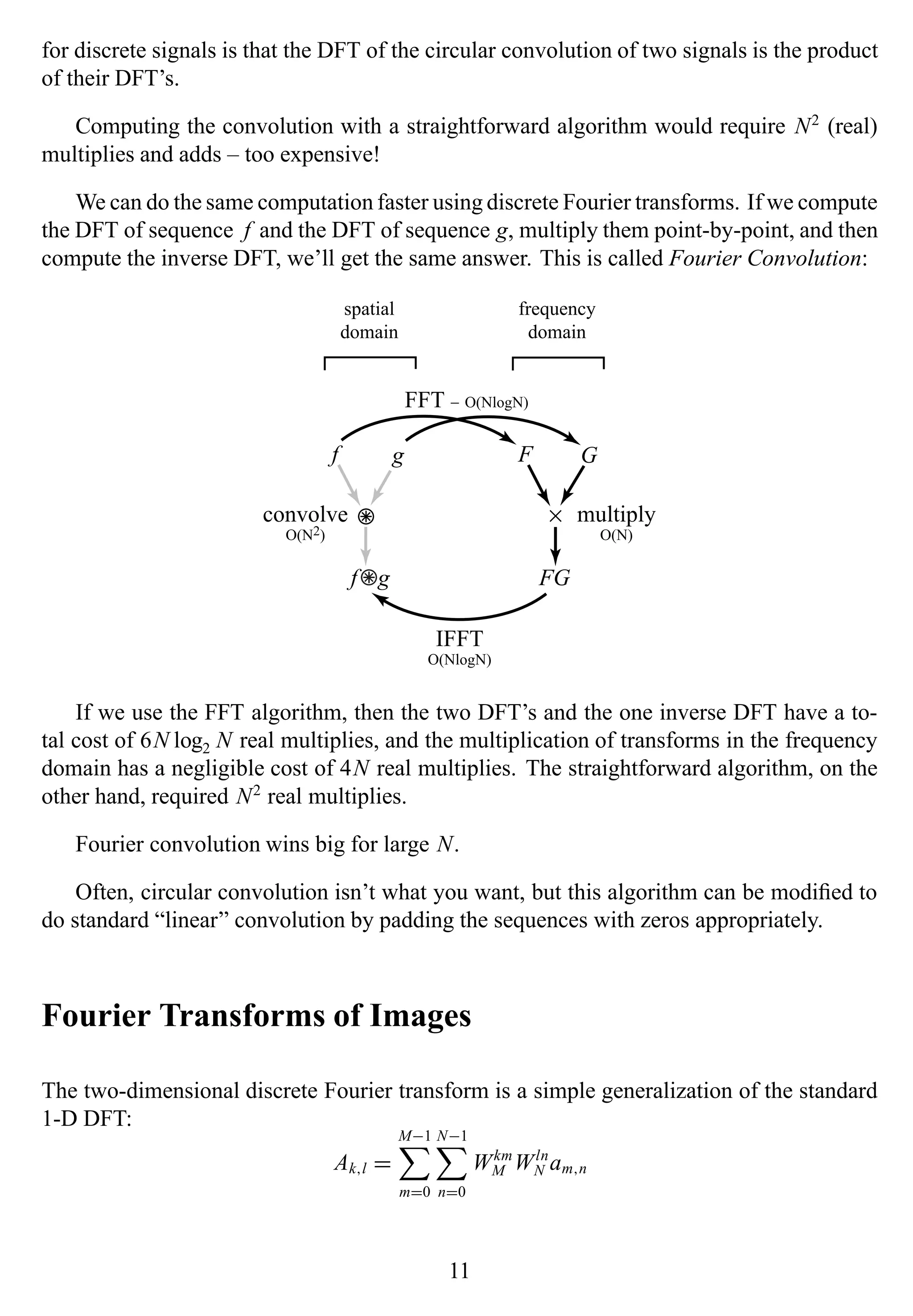
for discrete signalsis that the DFT of the circular convolution of two signals is the product
of their DFT’s.
Computing the convolution with a straightforward algorithm would require N2
(real)
multiplies and adds – too expensive!
We can do the same computation faster using discrete Fourier transforms. If we compute
the DFT of sequence f and the DFT of sequence g, multiply them point-by-point, and then
compute the inverse DFT, we’ll get the same answer. This is called Fourier Convolution:
f g
f⊕g
×
F G
FG
FFT − O(NlogN)
IFFT
O(NlogN)
convolve
O(N2)
multiply
O(N)
spatial
domain
frequency
domain
⊕⊗
⊗
If we use the FFT algorithm, then the two DFT’s and the one inverse DFT have a to-
tal cost of 6N log2 N real multiplies, and the multiplication of transforms in the frequency
domain has a negligible cost of 4N real multiplies. The straightforward algorithm, on the
other hand, required N2
real multiplies.
Fourier convolution wins big for large N.
Often, circular convolution isn’t what you want, but this algorithm can be modified to
do standard “linear” convolution by padding the sequences with zeros appropriately.
Fourier Transforms of Images
The two-dimensional discrete Fourier transform is a simple generalization of the standard
1-D DFT:
Ak,l =
M−1
m=0
N−1
n=0
Wkm
M Wln
N am,n
11
12.
This is thegeneral formula, good for rectangular images whose dimensions are not neces-
sarily powers of two. If you evaluate DFT’s of images with this formula, the cost is O(N4
)
– this is way too slow if N is large! But if you exploit the common subexpressions from row
to row, or from column to column, you get a speedup to O(N3
) (even without using FFT):
To compute the Fourier transform of an image, you
• Compute 1-D DFT of each row, in place.
• Compute 1-D DFT of each column, in place.
Most often, you see people assuming M = N = 2r
, but as mentioned previously, there
are FFT algorithms for other cases.
For an N × N picture, N a power of 2, the cost of a 2-D FFT is proportional to N2
log N.
( Can you derive this? ) Quite a speedup relative to O(N4
)!
Practical issues: For display purposes, you probably want to cyclically translate the pic-
ture so that pixel (0,0), which now contains frequency (ωx, ωy) = (0,0), moves to the center
of the image. And you probably want to display pixel values proportional to log(magnitude)
of each complex number (this looks more interesting than just magnitude). For color im-
ages, do the above to each of the three channels (R, G, and B) independently.
FFT’s are also used for synthesis of fractal textures and to create images with a given
spectrum.
Fourier Transforms and Arithmetic
The FFT is also used for fast extended precision arithmetic (e.g. computing π to a zillion
digits), and multiplication of high-degree polynomials, since they also involve convolution.
If polynomials p and q have the form: p(x) = N−1
n=0 fnxn
and q(x) = N−1
n=0 gnxn
then their
product is the polynomial
r(x) = p(x)q(x) =
N−1
n=0
fnxn
N−1
n=0
gnxn
= ( f0 + f1x + f2x2
+ ···)(g0 + g1x + g2x2
+ ···)
= f0g0 + ( f0g1 + f1g0)x + ( f0g2 + f1g1 + f2g0)x2
+ ···
=
2N−2
n=0
hnxn
12
13.
where hn =N−1
j=0 f jgn− j, and h = f ∗ g. Thus, computing the product of two polynomials
involves the convolution of their coefficient sequences.
Extended precision numbers (numbers with hundreds or thousands of significant figures)
are typically stored with a fixed number of bits or digits per computer word. This is equiv-
alent to a polynomial where x has a fixed value. For storage of 32 bits per word or 9 digits
per word, one would use x = 232
or 109
, respectively. Multiplication of extended preci-
sion numbers thus involves the multiplication of high-degree polynomials, or convolution
of long sequences.
When N is small (< 100, say), then straightforward convolution is reasonable, but for
large N, it makes sense to compute convolutions using Fourier convolution.
13
![for j = 0 to N-1
nj = bit_reverse(j)
if (j<nj) swap a[j] and a[nj]
General FFT and IFFT Algorithm for N = 2r
. The previously diagrammed algorithm
for the 8-point FFT is easily generalized to any power of two. The input array is bit-reversed,
and the butterfly coefficients can be seen to have exponents in arithmetic sequence modulo
N. For example, for N = 8, the butterfly coefficients on the last stage in the diagram are
W0
, W1
, W2
, W3
, W4
, W5
, W6
, W7
. That is, powers of W in sequence. The coefficients
in the previous stage have exponents 0,2,4,6,0,2,4,6, which is equivalent to the sequence
0,2,4,6,8,10,12,14 modulo 8. And the exponents in the first stage are 1,-1,1,-1,1,-1,1,-1,
which is equivalent to W raised to the powers 0,4,0,4,0,4,0,4, and this is equivalent to the
exponent sequence 0,4,8,12,16,20,24,28 when taken modulo 8. The width of the butterflies
(the height of the ”X’s” in the diagram) can be seen to be 1, 2, 4, ... in successive stages, and
the butterflies are seen to be isolated in the first stage (groups of 1), then clustered into over-
lapping groups of 2 in the second stage, groups of 4 in the 3rd stage, etc. The generalization
to other powers of two should be evident from the diagrams for N = 4 and N = 8.
The inverse FFT (IFFT) is identical to the FFT, except one exchanges the roles of a and
A, the signs of all the exponents of W are negated, and there’s a division by N at the end.
Note that the fast way to compute mod( j, N) in the C programming language, for N a power
of two, is with bit-wise AND: “j&(N-1)”. This is faster than “j%N”, and it works for
positive or negative j, while the latter does not.
FFT Explained Using Matrix Factorization
The 8-point DFT can be written as a matrix product, where we let W = W8 = e−iπ/4
= (1 −
i)/
√
2:
A0
A1
A2
A3
A4
A5
A6
A7
=
W0 W0 W0 W0 W0 W0 W0 W0
W0 W1 W2 W3 W4 W5 W6 W7
W0 W2 W4 W6 W0 W2 W4 W6
W0 W3 W6 W1 W4 W7 W2 W5
W0 W4 W0 W4 W0 W4 W0 W4
W0 W5 W2 W7 W4 W1 W6 W3
W0 W6 W4 W2 W0 W6 W4 W2
W0 W7 W6 W5 W4 W3 W2 W1
a0
a1
a2
a3
a4
a5
a6
a7
8](https://image.slidesharecdn.com/fouriertransformsfftalgorithmpaulheckbert1998bytantanoid-130608110825-phpapp02/75/Fourier-transforms-fft-algorithm-paul-heckbert-1998-by-tantanoid-8-2048.jpg)
![There are N/2 butterflies per stage, and log2 N stages, so that means about 4 · N/2 ·
log2 N = 2N log2 N real multiplies and 3N log2 N real adds for an N-point FFT. (There are
ways to optimize further, but this is the basic FFT algorithm.)
Cost comparison:
BRUTE FORCE FFT
N r = log2 N 4N2
2N log2 N speedup
2 1 16 4 4
4 2 64 16 4
8 3 256 48 5
1,024 10 4,194,304 20,480 205
65,536 16 1.7 · 1010
2.1 · 106
˜104
The FFT algorithm is a LOT faster for big N.
There are also FFT algorithms for N not a power of two. The algorithms are generally
fastest when N has many factors, however.
An excellent book on the FFT is: E. Oran Brigham, The Fast Fourier Transform, Prentice-
Hall, Englewood Cliffs, NJ, 1974.
Why Would We Want to Compute Fourier Transforms, Any-
way?
The FFT algorithm is used for fast convolution(linear, shift-invariant filtering). If h = f ∗ g
then convolution of continuous signals involves an integral:
h(x) =
+∞
−∞
f (t)g(x − t)dt, but convolution of discrete signals involves a sum: h[x] =
∞
t=−∞ f [t]g[x − t]. We might think of f as the signal and g as the filter.
When working with finite sequences, the definition of convolution simplifies if we as-
sume that f and g have the same length N and we regard the signals as being periodic, so
that f and g “wrap around”. Then we get circular convolution:
h[x] =
N−1
t=0
f [t]g[x − t mod N] for x = 0. . . N − 1
The convolution theorem says that the Fourier transform of the convolution of two sig-
nals is the product of their Fourier transforms: f ∗ g ↔ FG. The corresponding theorem
10](https://image.slidesharecdn.com/fouriertransformsfftalgorithmpaulheckbert1998bytantanoid-130608110825-phpapp02/75/Fourier-transforms-fft-algorithm-paul-heckbert-1998-by-tantanoid-10-2048.jpg)