![Discrete Time FT (DTFT)
DTFT defined as: Note: continuous frequency domain!
(frequency density function)
s
si +∞
ly
na
a S(f) = ∑ s[n] ⋅ e − j 2 π f n
n = −∞ Holds for Aperiodic
signals
is
hes 2π
nt 1
sy s[n] = ⋅ ∫ S(f)e j 2 π f ndf
2π
0](https://image.slidesharecdn.com/finalpresentationdft-121117110039-phpapp02/75/Discrete-Fourier-Transform-2-2048.jpg)
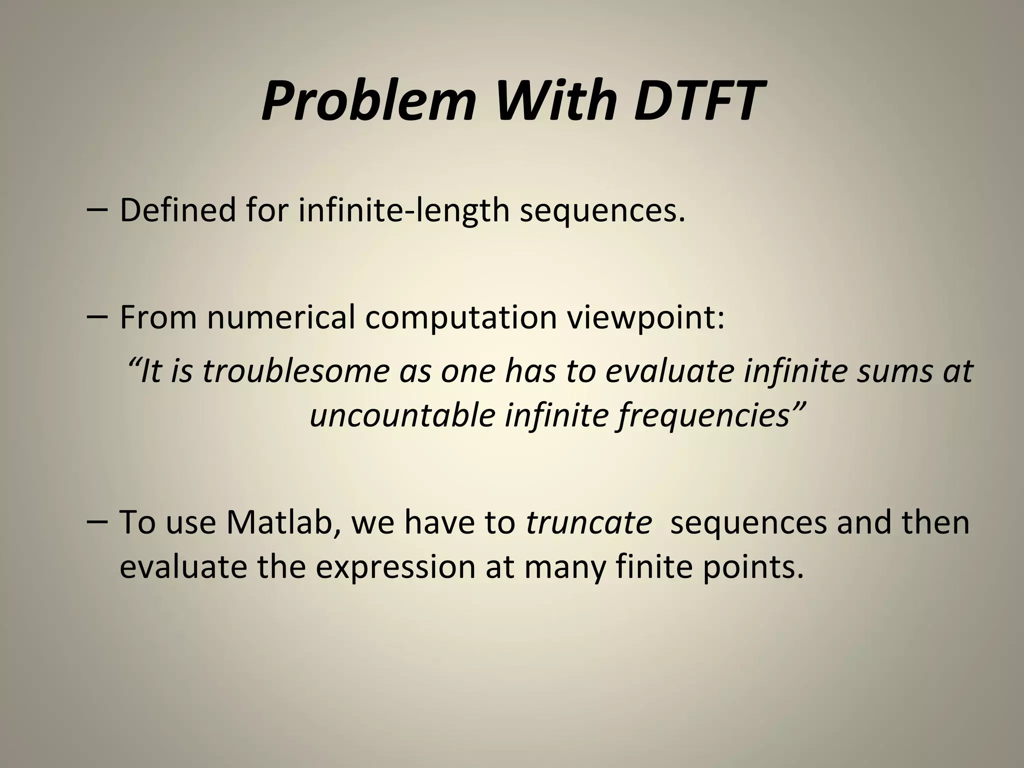
![Discrete Fourier Series
Analysis equation:
~ N −1
~[n]e − j( 2 π / N)kn
X[k ] = ∑x
n=0
Synthesis equation:
~[n] = 1 N −1 ~
x ∑ X[k ]e j( 2 π / N)kn
N k =0](https://image.slidesharecdn.com/finalpresentationdft-121117110039-phpapp02/75/Discrete-Fourier-Transform-6-2048.jpg)
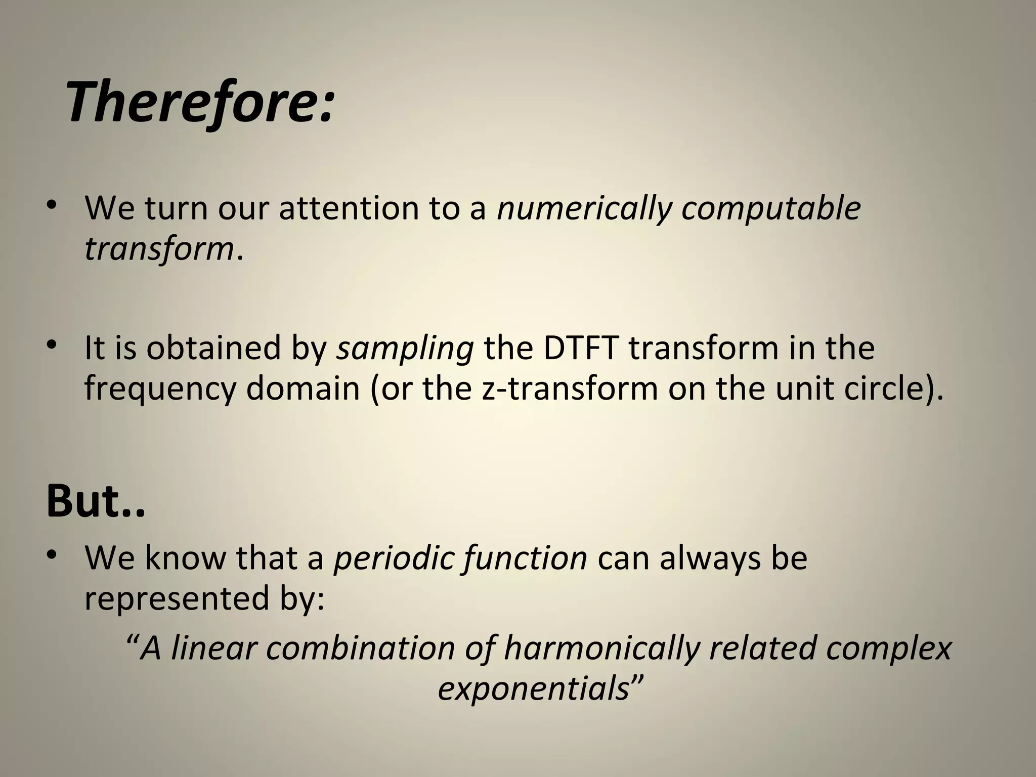
![• For convenience we sometimes use:
− j( 2 π / N )
WN = e
So..
~ N −1
~[n]Wkn
X[k ] = ∑x N
n=0
~
{ X ( K ), k = 0,±1, } called the discrete Fourier series
are
coefficients.
~[n] = 1
N −1
~
x ∑ X[k ]WN kn
−
N k =0](https://image.slidesharecdn.com/finalpresentationdft-121117110039-phpapp02/75/Discrete-Fourier-Transform-7-2048.jpg)
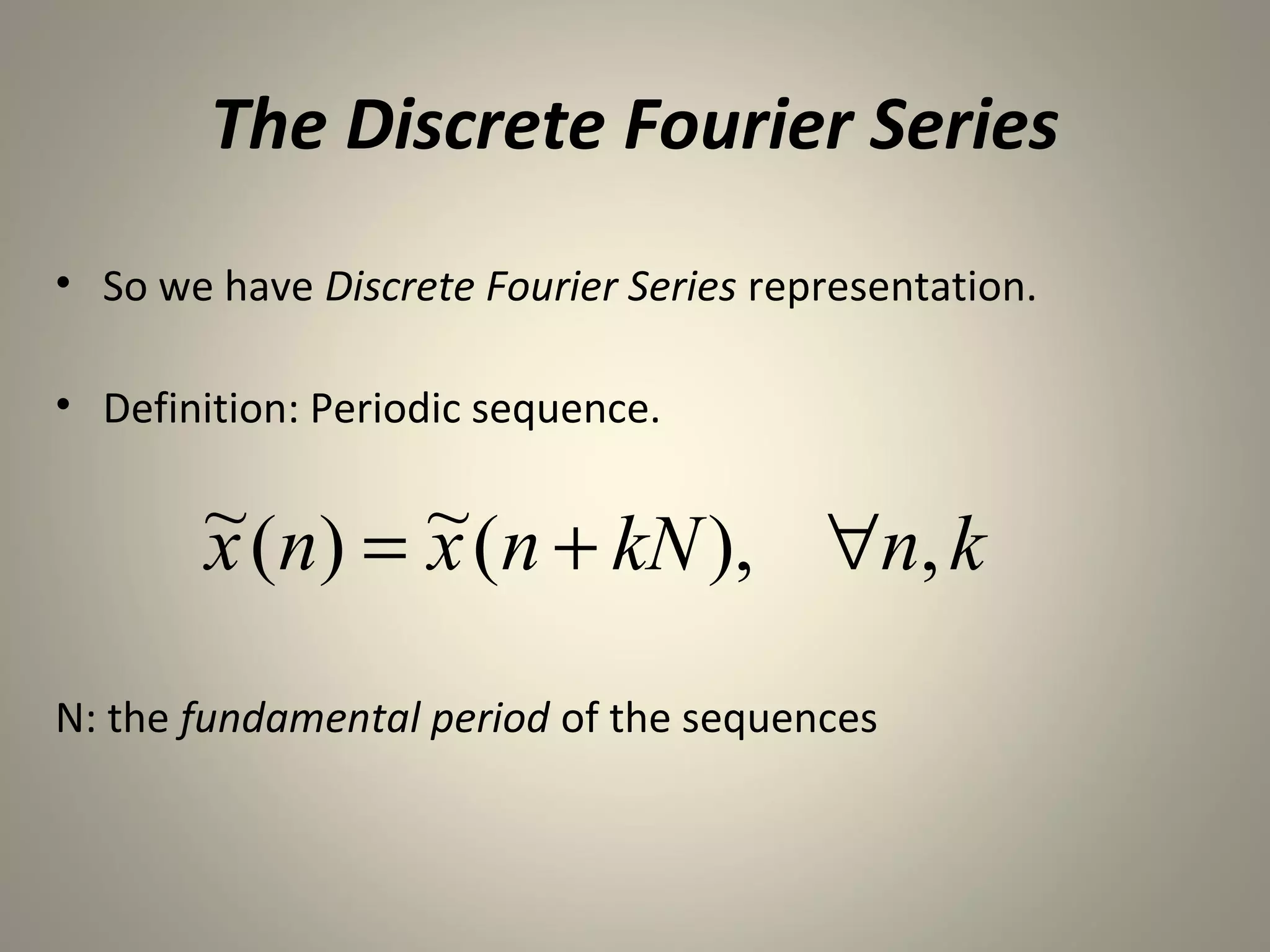
![Properties of DFS
• Linearity
~ [n] ~
x1 ← DFS →
X1 [k ]
~ [n] ~
x 2 ← DFS →
X2 [k ]
~ ~
a~1 [n] + b~2 [n]
x x ← DFS → aX1 [k ] + bX2 [k ]
• Shift of a Sequence
~[n] ~
x ← DFS →
X[k ]
~
X[n] ← DFS → N~[ − k ]
x
• Duality
~[n] ~
x DFS
← →
X[k ]
~[n − m] ~
x ← → e − j2 πkm / NX[k ]
DFS
e j2 πnm / N~
x [n] ← → ~[k − m]
DFS
X](https://image.slidesharecdn.com/finalpresentationdft-121117110039-phpapp02/75/Discrete-Fourier-Transform-8-2048.jpg)
![DFT Properties
Time Frequency
Linearity a·s[n] + b·u[n] a·S(k)+b·U(k)
1 N−1
Multiplication s[n] ·u[n] ⋅ ∑S(h)U(k - h)
N h =0
N− 1
Convolution S(k)·U(k)
∑ s[m] ⋅ u[n − m]
m= 0
Time shifting s[n - m]
2π k ⋅m
−j
e T ⋅ S(k)
Frequency shifting S(k - h)
2π h t
+j
e T ⋅ s[n]](https://image.slidesharecdn.com/finalpresentationdft-121117110039-phpapp02/75/Discrete-Fourier-Transform-17-2048.jpg)
![s[n]
S(f)
(a) (b)
0 T/2 T 2T f
s”[n] IDFT
DFT
(c) (d)
(e)
(f) cK
(a) Aperiodic discrete signal. (b) DTFT transform magnitude.
(c) Periodic version of (a). (d) DFS coefficients = samples of (b).
(e) Inverse DFT estimates a single period of s[n]
(f) DFT estimates a single period of (d).](https://image.slidesharecdn.com/finalpresentationdft-121117110039-phpapp02/75/Discrete-Fourier-Transform-18-2048.jpg)


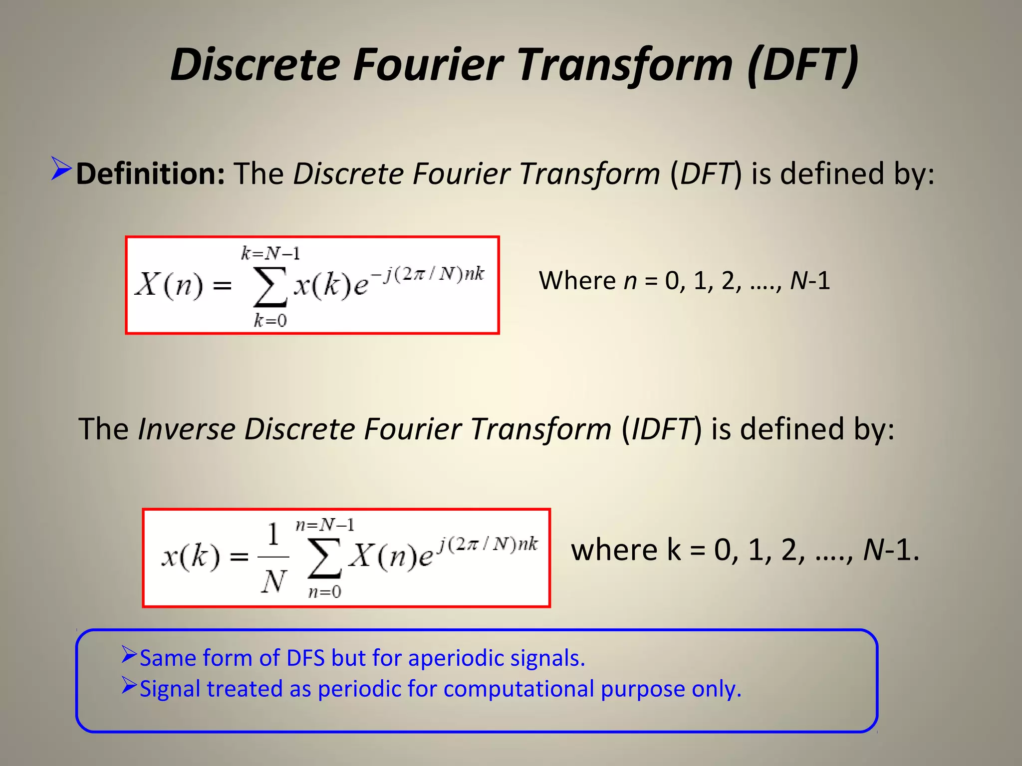
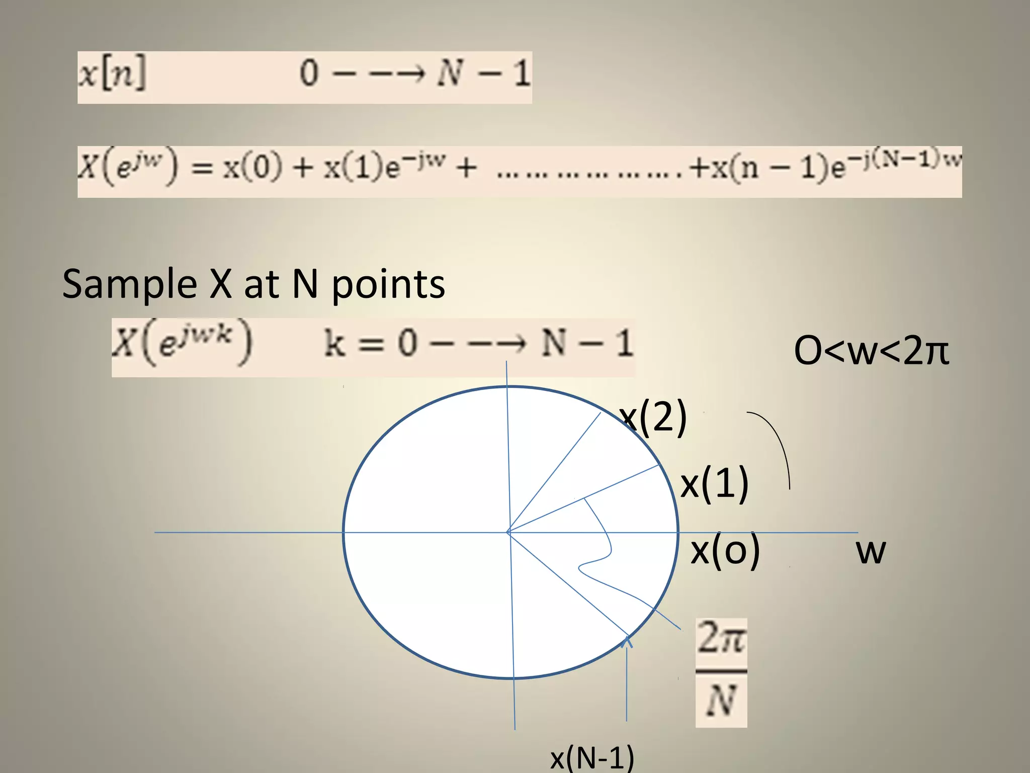
The document discusses the Discrete Fourier Transform (DFT). It begins by explaining the limitations of the Discrete Time Fourier Transform (DTFT) and Discrete Fourier Series (DFS) from a numerical computation perspective. It then introduces the DFT as a numerically computable transform obtained by sampling the DTFT in the frequency domain. The DFT represents a periodic discrete-time signal using a sum of complex exponentials. It defines the DFT and inverse DFT equations. The document also discusses properties of the DFT such as linearity and time/frequency shifting. Finally, it notes that the Fast Fourier Transform (FFT) implements the DFT more efficiently by constraining the number of points to powers of two.