Downloaded 19 times
![1 The Spectrum of a Stationary Process
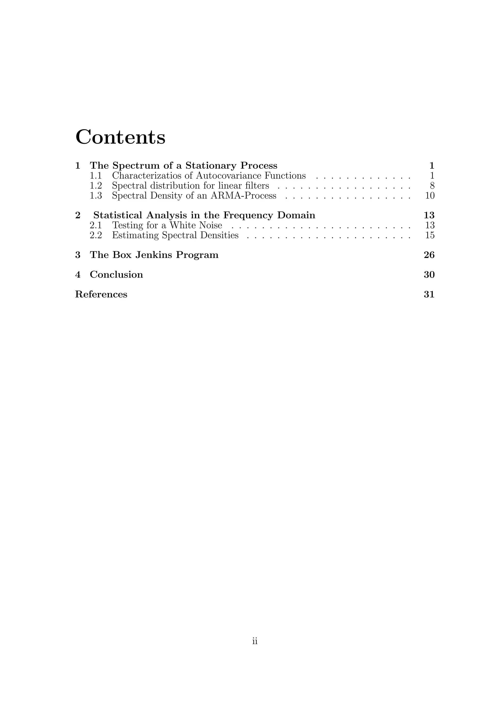
Theorem 1.1.2. A symmetric function K : Z −→ R is positive semidefinite iff it
can be represented as an integral
γ(h) =
1
0
ei2πλh
dF(λ) =
1
0
cos(2πλh)dF(λ),
where F is a real valued measure generating function on [0, 1] with F(0) = 0. The
function F is uniquely determined.
Proof. We establish first the uniqueness of F. Let G be another measure generating
function with G(λ) = 0 for λ ≤ 0 and constant for λ ≥ 1 such that
γ(h) =
1
0
ei2πλh
dF(λ) =
1
0
ei2πλh
dG(λ) , h ∈ Z.
Let now ψ be a continuous function on [0, 1]. From calculus we know that we can find
for arbitrary ε > 0 a trigonometric polynomial pε(λ) = N
h=−N ahei2πλh
, 0 ≤ λ ≤ 1,
such that
sup
0≤λ≤1
|ψ(λ) − pε(λ)| ≤ ε.
As a consequence we obtain that
1
0
ψ(λ)dF(λ) =
1
0
pε(λ)dF(λ) + r1(ε)
=
1
0
pε(λ)dG(λ) + r1(ε)
=
1
0
ψ(λ)dG(λ) + r2(ε)
where ri(ε) → 0 as ε → 0, i = 1, 2, and, thus,
1
0
ψ(λ)dF(λ) =
1
0
ψ(λ)dG(λ).
Since ψ was an arbitrary continuous function, this in turn together with F(0) =
G(0) = 0 implies F = G. Suppose now that γ has the representation
γ(h) =
1
0
ei2πλh
dF(λ) =
1
0
cos(2πλh)dF(λ)
4](https://image.slidesharecdn.com/kavitay1011021-140530015246-phpapp01/75/Time-Series-Analysis-7-2048.jpg)
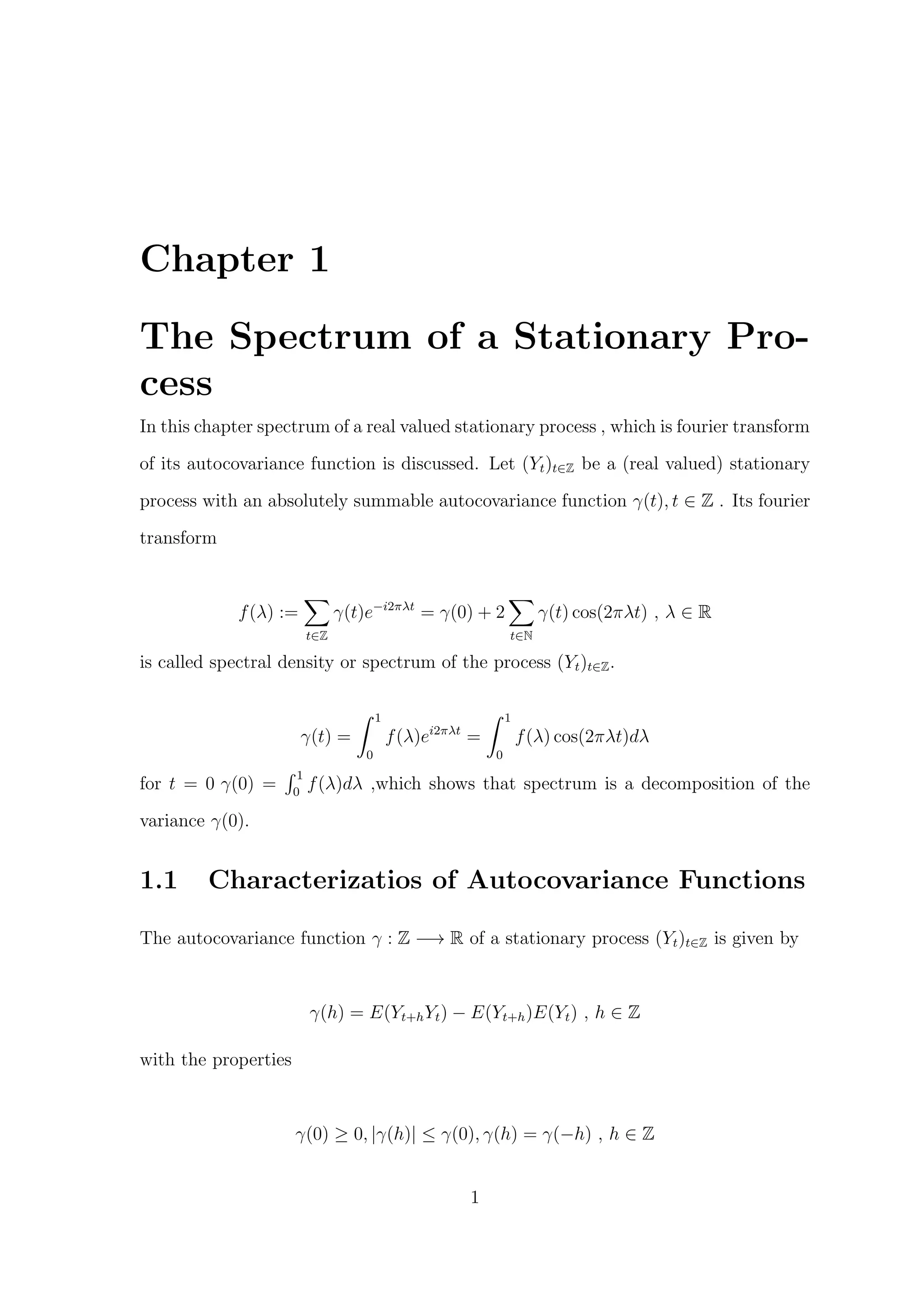
![1 The Spectrum of a Stationary Process
We have for arbitrary xi ∈ R, i = 1, ..., n
1≤r,s≤n
xrγ(r − s)xs =
1
0 1≤r,s≤n
xrxsei2πλ(r−s)
dF(λ)
=
1
0
|
n
r=1
xrei2πλr
|2
dF(λ) ≥ 0,
i.e., γ is positive semidefinite. Suppose conversely that γ : Z −→ R is a positive
semidefinite function. This implies that for 0 ≤ λ ≤ 1 and N ∈ N
fN (λ) :=
1
N 1≤r,s≤N
e−i2πλr
γ(r − s)ei2πλs
=
1
N
|m|<N
(N − |m|)γ(m)e−i2πλm
≥ 0
Put now
FN (λ) :=
λ
0
fN (x)dx, 0 ≤ λ ≤ 1.
Then we have for each h ∈ Z
1
0
ei2πλh
=
|m|<N
1 −
|m|
N
γ(m)
1
0
ei2πλ(h−m)
dλ
=
1 − |m|
N
γ(m) if |h| < N
0, if |h| ≥ N
Since FN (1) = γ(0) < ∞ for any N ∈ N, we can apply Helly’s selection theorem to
deduce the existence of a measure generating function ˜F and a subsequence (FNk
)k
such that FNk
converges weakly to ˜F i.e.,
1
0
g(λ)dFNk
(λ)
k→∞
−−−→
1
0
g(λ)d ˜F(λ)
for every continuous and bounded function g : [0, 1] −→ R. Put now F(λ) :=
˜F(λ) − ˜F(0). Then F is a measure generating function with F(0) = 0 and
1
0
g(λ)d ˜F(λ) =
1
0
g(λ)dF(λ).
5](https://image.slidesharecdn.com/kavitay1011021-140530015246-phpapp01/75/Time-Series-Analysis-8-2048.jpg)
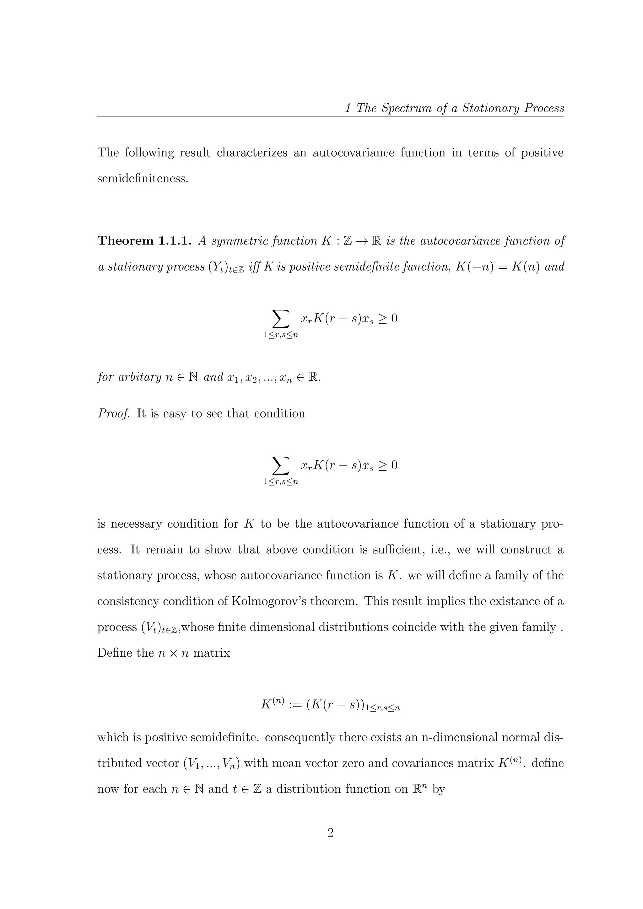
![1 The Spectrum of a Stationary Process
If we replace N in
1
0
ei2πλh
=
|m|<N
1 −
|m|
N
γ(m)
1
0
ei2πλ(h−m)
dλ
=
1 − |m|
N
γ(m) if |h| < N
0, if |h| ≥ N
by Nk and let k tend to infinity, we now obtain representation desired.
Example 1.1.1. A white noise (εt)tinZ has the autocovariance function
γ(h) =
σ2
, if h = 0
0, if h ∈ Z {0}
Since
1
0
σ2
ei2πλh
dλ =
σ2
, if h = 0
0, if h ∈ Z {0}
the process (εt) has by Theorem 1.1.2 the constant spectral density f(λ) = σ2
, 0 ≤
λ ≤ 1. This is the name giving property of the white noise process: As the white
light is characteristically perceived to belong to objects that reflect nearly all incident
energy throughout the visible spectrum, a white noise process weighs all possible
frequencies equally.
Corollary 1.1.3. A symmetric function γ : Z −→ R is the autocovariance function
of a stationary process (Yt)t∈Z, iff it satisfies one of the following two (equivalent)
conditions:
(i) γ(h) =
1
0
ei2πλh
dF(λ), h ∈ Z, where F is a measure generating function on [0, 1]
with F(0) = 0.
(ii) 1≤r,s≤n xrγ(r − s)xs ≥ 0 for each n ∈ N and x1, ..., xn ∈ R.
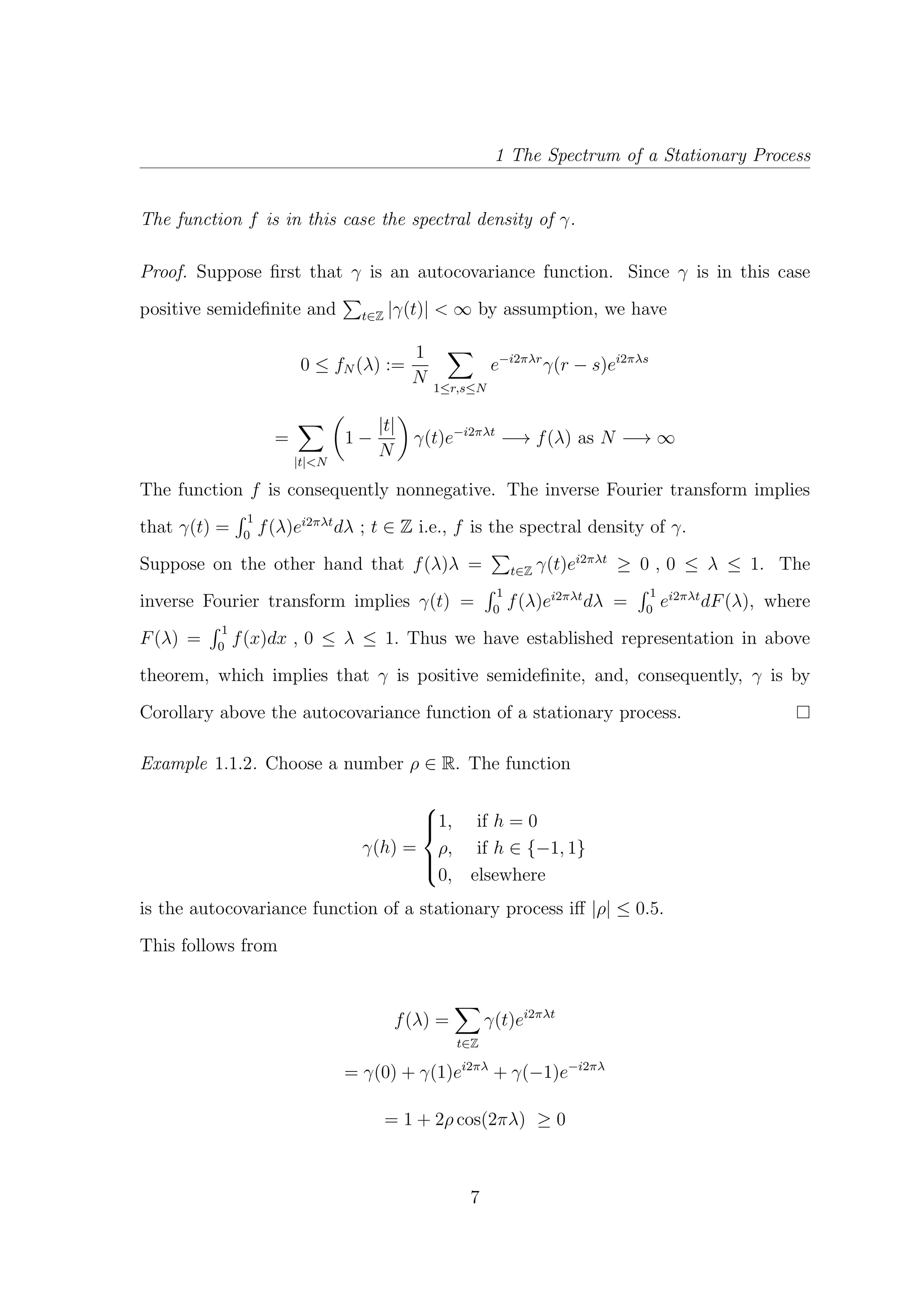
Corollary 1.1.4. A symmetric function γ : Z −→ R with t∈Z |γ(t)| < ∞ is the
autocovariance function of a stationary process iff
f(λ) :=
t∈Z
γ(t)e−i2πλt
≥ 0 , λ ∈ [0, 1]
6](https://image.slidesharecdn.com/kavitay1011021-140530015246-phpapp01/75/Time-Series-Analysis-9-2048.jpg)
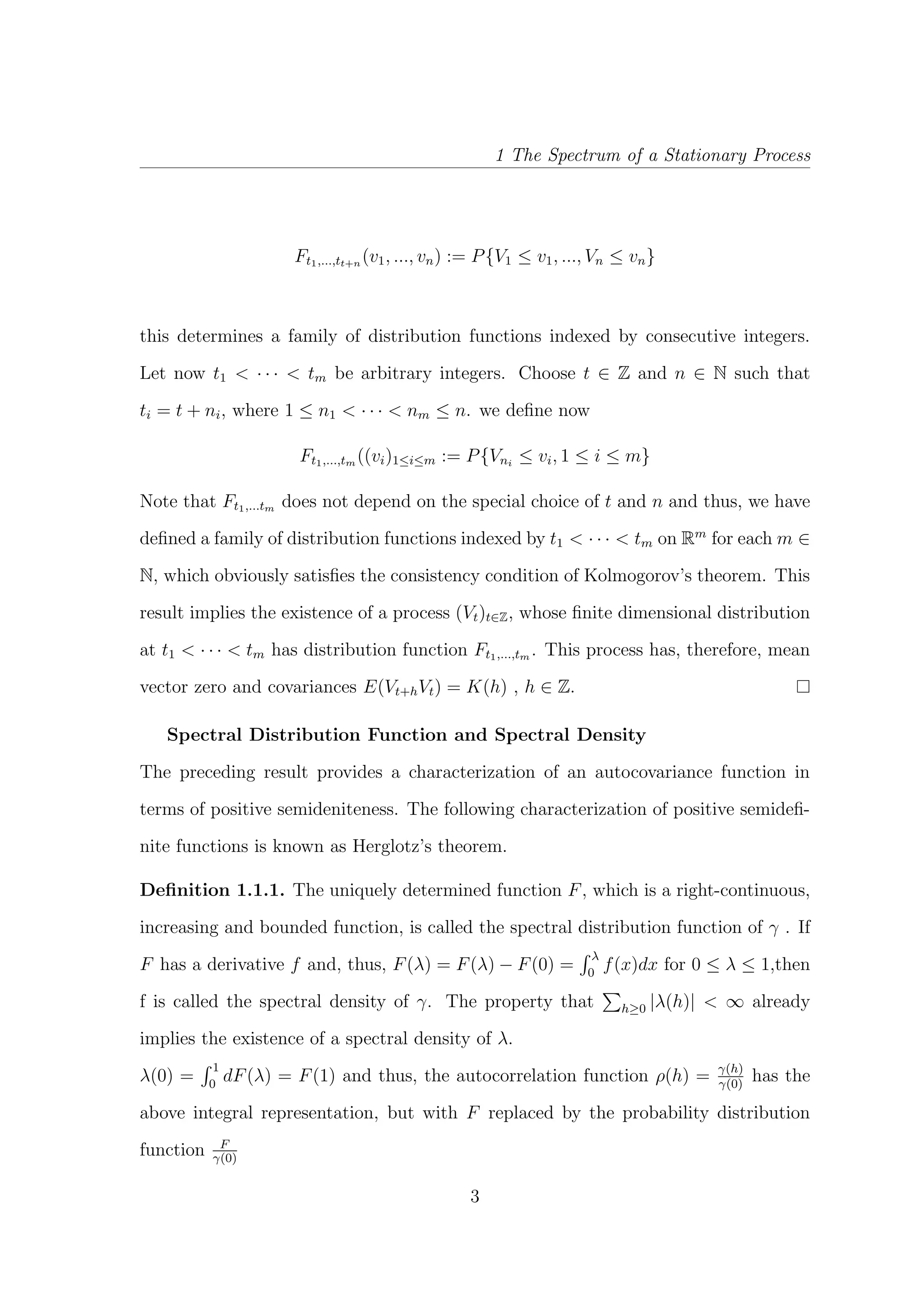
![1 The Spectrum of a Stationary Process
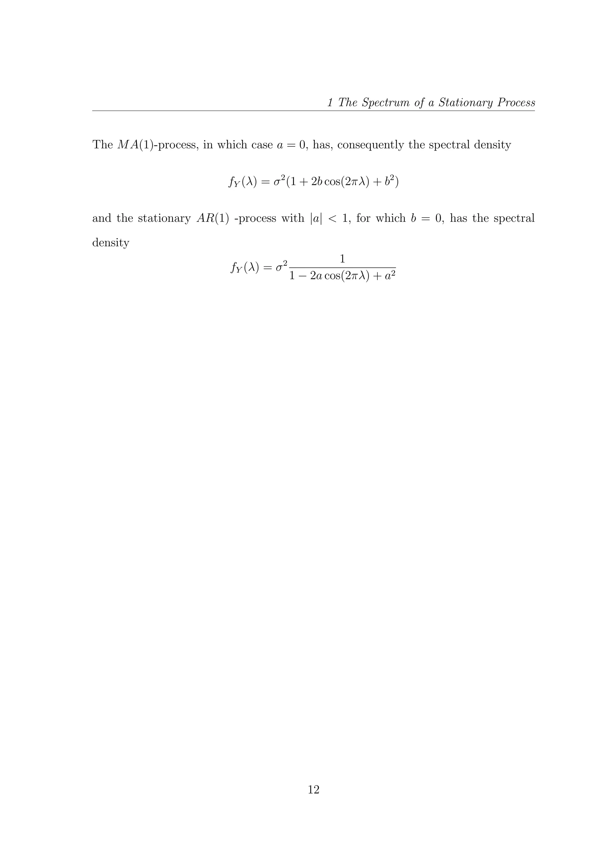
for λ ∈ [0, 1] iff |ρ| ≤ 0.5. The function γ is the autocorrelation function of an
MA(1)-process. The spectral distribution function of a stationary process satisfies
F(0.5 + λ) − F(0.5−
) = F(0.5) − F((0.5 − λ)−
) , 0 ≤ λ < 0.5,
where F(x−
) := limε↓0F(x − ε) is the left-hand limit of F at x ∈ (0, 1] . If F has
a derivative f, we obtain from the above symmetry f(0.5 + λ) = f(0.5 − λ) or,
equivalently, f(1λ) = f(λ) and, hence,
γ(h) =
1
0
cos(2πλh)dF(λ) = 2
0.5
0
cos(2πλh)f(λ)df(λ)
The autocovariance function of a stationary process is, therefore, determined by the
values f(λ) , 0 ≤ λ ≤ 0.5, if the spectral density exists. Moreover, that the smallest
nonconstant period P0 visible through observations evaluated at time points t =
1, 2, ... is P0 = 2 i.e., the largest observable frequency is the Nyquist frequency λ0 =
1
P0
= 0.5, Hence, the spectral density f(λ) matters only for λ ∈ [0, 0.5].
Remark 1.1.1. The preceding Theorems shows that a function f : [0, 1] −→ R is the
spectral density of a stationary process iff f satisfies the following three conditions
(i)f(λ) ≥ 0,
(ii)f(λ) = f(1 − λ),
(iii)
1
0
f(λ)dλ < ∞
1.2 Spectral distribution for linear filters
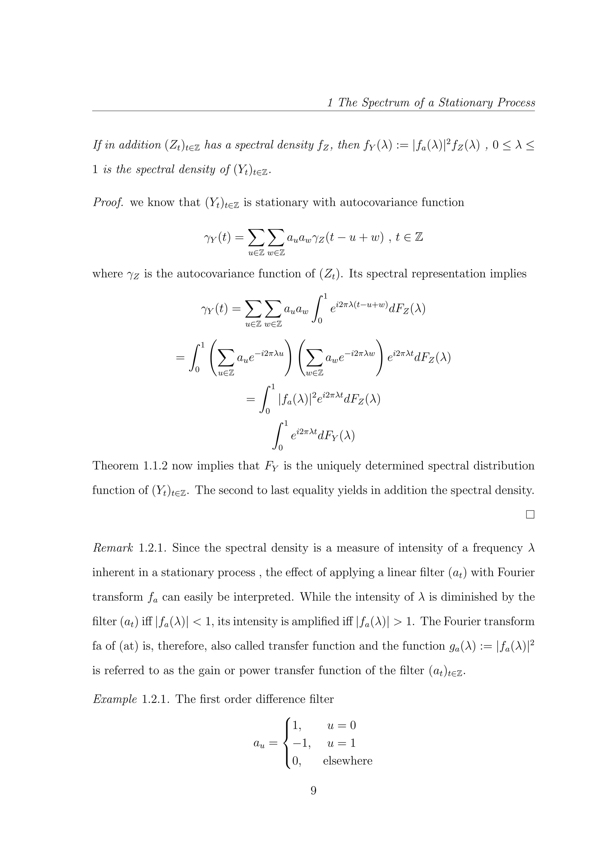
Theorem 1.2.1. Let (Zt)t∈Z be a stationary process with spectral distribution function
FZ and let (at)t∈Z be an absolutely summable filter with Fourier transform fa. The
linear filtered process Yt := u∈Z auZt−u, t ∈ Z then has the spectral distribution
function
FY (λ) :=
1
0
|fa(x)|2
dFZ(x) , 0 ≤ λ ≤ 1.
8](https://image.slidesharecdn.com/kavitay1011021-140530015246-phpapp01/75/Time-Series-Analysis-11-2048.jpg)
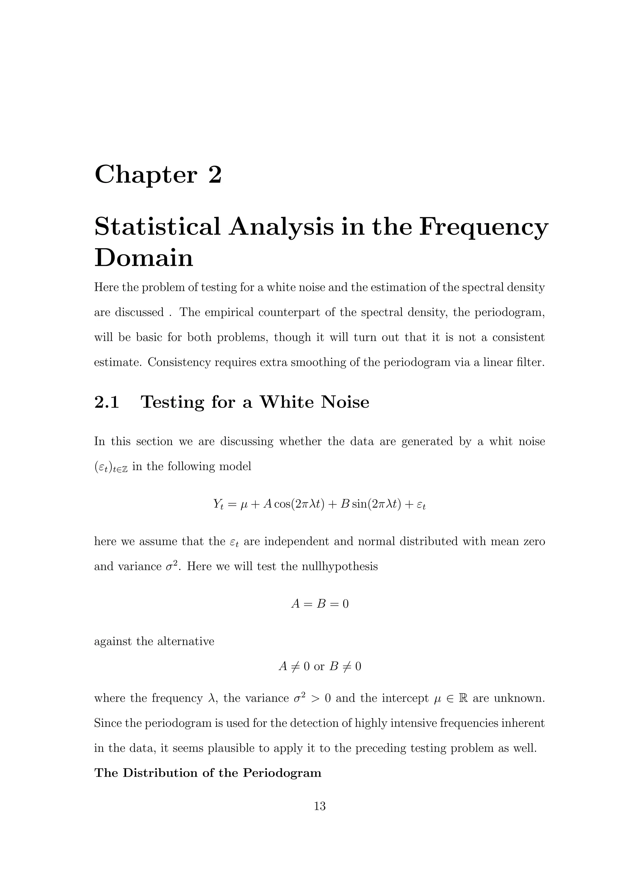
![2 Statistical Analysis in the Frequency Domain
Lemma 2.1.1. Let ε1, ..., εn be independent and identically normal distributed random
variables with mean µ ∈ R and variance σ2
> 0. Denote by ¯ε := 1
n
n
t=1 εt the sample
mean of ε1, ..., εn and by
Cε (k/n) =
1
n
n
t=1
(εt − ¯ε) cos 2
k
n
t
Sε (k/n) =
1
n
n
t=1
(εt − ¯ε) sin 2
k
n
t
the cross covariances with Fourier frequencies k/n , 1 ≤ k ≤ [(n − 1)/2]. Then the
2[(n − 1)/2] random variables
Cε (k/n) , Sε (k/n) , 1 ≤ k ≤ [(n − 1)/2]
are independent and identically N(0, σ2
/(2n))-distributed.
Corollary 2.1.2. Let ε1, ..., εn be as in the preceding lemma and let
Iε (k/n) = n C2
ε (k/n) + S2
ε (k/n)
be the pertaining periodogram, evaluated at the Fourier frequencies k/n , 1 ≤ k ≤
[(n−1)/2] , k ∈ N .The random variables Iε(k/n)/σ2
are independent and identically
standard exponential distributed i.e.,
P Iε(k/n)/σ2
≤ x =
1 − exp(−x) , x > 0
0 , x ≤ 0
Proof. Lemma mentioned above implies that
2n
σ2
Cε(k/n) ,
2n
σ2
Sε(k/n)
are independent standard normal random variables and, thus,
2Iε(k/n)
σ2
=
2n
σ2
Cε(k/n)
2
+
2n
σ2
Sε(k/n)
2
is χ2
-distributed with two degrees of freedom. Since this distribution has the distri-
bution function 1 − exp(−x/2) , x ≤ 0, the assertion follows.
14](https://image.slidesharecdn.com/kavitay1011021-140530015246-phpapp01/75/Time-Series-Analysis-17-2048.jpg)
![2 Statistical Analysis in the Frequency Domain
For testing of White noise following test are used :
Fisher’s Test
κm :=
max1≤j≤m I(j/n)
(1/m) m
k=1 I(k/n)
= mMm
Where Mm :=
max1≤j≤m Iε(j/n)
m
k=1 Iε(k/n)
is significantly large, i.e., if one of the values I(j/n) is
significantly larger than the average over all. The hypothesis ( data is generated by
white noise ) is, therefore, rejected at error level α if
κm > cα with 1 − Gm
cα
m
= α
The BartlettKolmogorovSmirnov Test
The KolmogorovSmirnov statistic
∆m−1 := sup
x∈[0,1]
| ˆFm−1(x) − x|
In this test we fit our data points with graph of x and if value of ∆ is too high then
hypothesis is rejected.
2.2 Estimating Spectral Densities
We are assuming in the following that (Yt)t∈Z is a stationary real valued process with
mean µ and absolutely summable autocovariance function γ. From last chapter we
know that the process (Yt)t∈Z has the continous spectral density
f(λ) =
h∈Z
γ(h)e−i2πλh
In this section we will invetigate the limit behaviour of the periodogram for arbitrary
independent random variable (Yt)
Asymptotic Properties of the Periodogram
For Fourier frequencies k/n , 0 ≤ k ≤ [n/2] we put
In(k/n) =
1
n
|
n
t=1
Yte−i2π(k/n)t
|2
15](https://image.slidesharecdn.com/kavitay1011021-140530015246-phpapp01/75/Time-Series-Analysis-18-2048.jpg)
![2 Statistical Analysis in the Frequency Domain
=
1
n
n
t=1
Yt cos(2π
k
n
t)
2
+
n
t=1
Yt sin(2π
k
n
t)
2
Up to k = 0, this coincide with the definition of the periodogram and it have repre-
sentation
In(k/n) ==
n¯Y 2
n , k = 0
|h|<n c(h)e−i2π(k/n)h
, k = 1, ..., [n/2]
with ¯Yn := 1
n
n
t=1 Yt and the sample autocovariance function
c(h) =
1
n
n−|h|
t=1
(Yt − ¯Yn)(Yt+|h| − ¯Yn)
By above representation , the results related to periodogarm done earlier and the
value In(k/n) does not change for k = 0 if we replace sample mean ¯Yn in c(h) by the
theoretical mean µ. This leads to the equivalent representation of the periodogram
for k = 0
In(k/n) =
|h|<n
1
n
n−|h|
t=1
(Yt − µ)(Yt+|h| − µ)
e−i2π(k/n)h
=
1
n
n
t=1
(Yt − µ) + 2
n−1
h=1
1
n
n−|h|
t=1
(Yt − µ)(Yt+|h| − µ)
cos(2π
k
n
h)
We define now the periodogram for λ ∈ [0, 0.5] as a piecewise constant function
In(λ) = In(k/n) if
k
n
−
1
2n
< λ ≤
k
n
+
1
2n
The following result shows that the periodogram In(λ) is for λ = 0 an asymptotically
unbiased estimator of the spectral density f(λ).
Theorem 2.2.1. Let (Yt)t∈Z be a stationary process with absolutely summable auto-
covariance function γ . Then we have with µ = E(Yt)
E(In(0)) − nµ2 n→∞
−−−→ f(0),
E(In(λ))
n→∞
−−−→ f(λ) , λ = 0
If λ = 0, then the convergence E(In(λ))
n→∞
−−−→ f(λ) holds uniformly on [0.0.5].
16](https://image.slidesharecdn.com/kavitay1011021-140530015246-phpapp01/75/Time-Series-Analysis-19-2048.jpg)
![2 Statistical Analysis in the Frequency Domain
Proof. By representation written above the theorem and the Cesaro convergence re-
sult we have
E(In(0)) − nµ2
=
1
n
n
t=1
n
s=1
E(YtYs) − nµ2
=
1
n
n
t=1
n
s=1
Cov(Ys, Yt)
=
|h|<n
1 −
|h|
n
γ(h)
n→∞
−−−→
h∈Z
γ(h) = f(0)
Define now for λ ∈ [0, 0, 5] the auxiliary function
gn(λ) :=
k
n
, if
k
n
−
1
2n
< λ ≤
k
n
+
1
2n
Then we obviously have
In(λ) = In(gn(λ))
Choose now λ ∈ (0, 0.5]. Since gn(λ) −→ λasn −→ ∞, it follows that gn(λ) > 0 for
n large enough. now we obtain for such n
E(In(λ)) =
|h|<n
1
n
n−|h|
t=1
E (Yt − µ)(Yt+|h| − µ) e−i2πgn(λ)h
=
|h|<n
1 −
|h|
n
γ(h)e−i2πgn(λ)h
Since h∈Z |γ(h)| < ∞, the series |h|<n γ(h) exp(−i2πλh) converges to f(λ) uni-
formly for 0 ≤ λ ≤ 0.5. Kronecker’s implies moreover
|
|h|<n
|h|
n
γ(h)e−i2πλh
| ≤
|h|<n
|h|
n
|γ(h)|
n→∞
−−−→ 0
and, thus, the series
fn(λ) :=
|h|<n
1 −
|h|
n
γ(h)e−i2πλh
17](https://image.slidesharecdn.com/kavitay1011021-140530015246-phpapp01/75/Time-Series-Analysis-20-2048.jpg)
![2 Statistical Analysis in the Frequency Domain
converges to f(λ) uniformly in λ as well. From gn(λ)
n→∞
−−−→ λ and the continuity of
f we obtain for λ ∈ (0, 0, 5]
|E(In(λ)) − f(λ)| = |fn(gn(λ)) − f(λ)|
≤ |fn(gn(λ)) − f(gn(λ))| + |f(gn(λ)) − f(λ)|
n→∞
−−−→ 0
Note that |gn(λ) − λ| ≤ 1/(2n). The uniform convergence in case of µ = 0 then
follows from the uniform convergence of gn(λ) to λ and the uniform continuity of f
on the compact interval [0, 0.5].
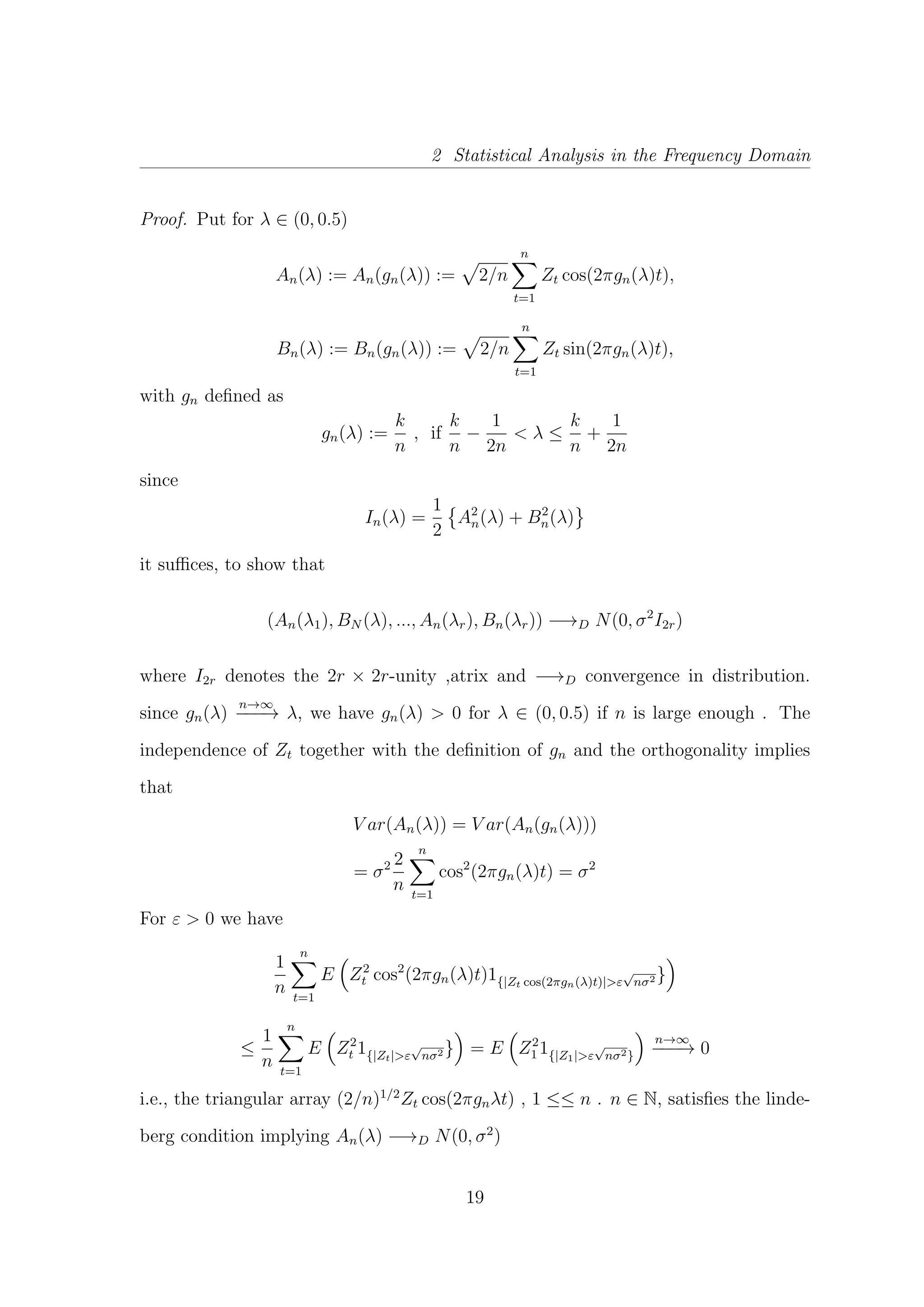
Theorem 2.2.2. Let Z1, ..., Zn be independent and identically distributed random
variables with mean E(Zt) = 0 and variance E(Z2
t ) = σ2
< ∞. Denote by In(λ) the
pertaining periodogram as defined earlier (In(λ) = In(gn(λ))).
(i) The random vector (In(λ1), ..., In(λr)) with 0 < λ1 < ... < λr < 0.5 converges in
distribution for n −→ ∞ to the distribution of r independent and identically expo-
nential distributed random variables with mean σ2
.
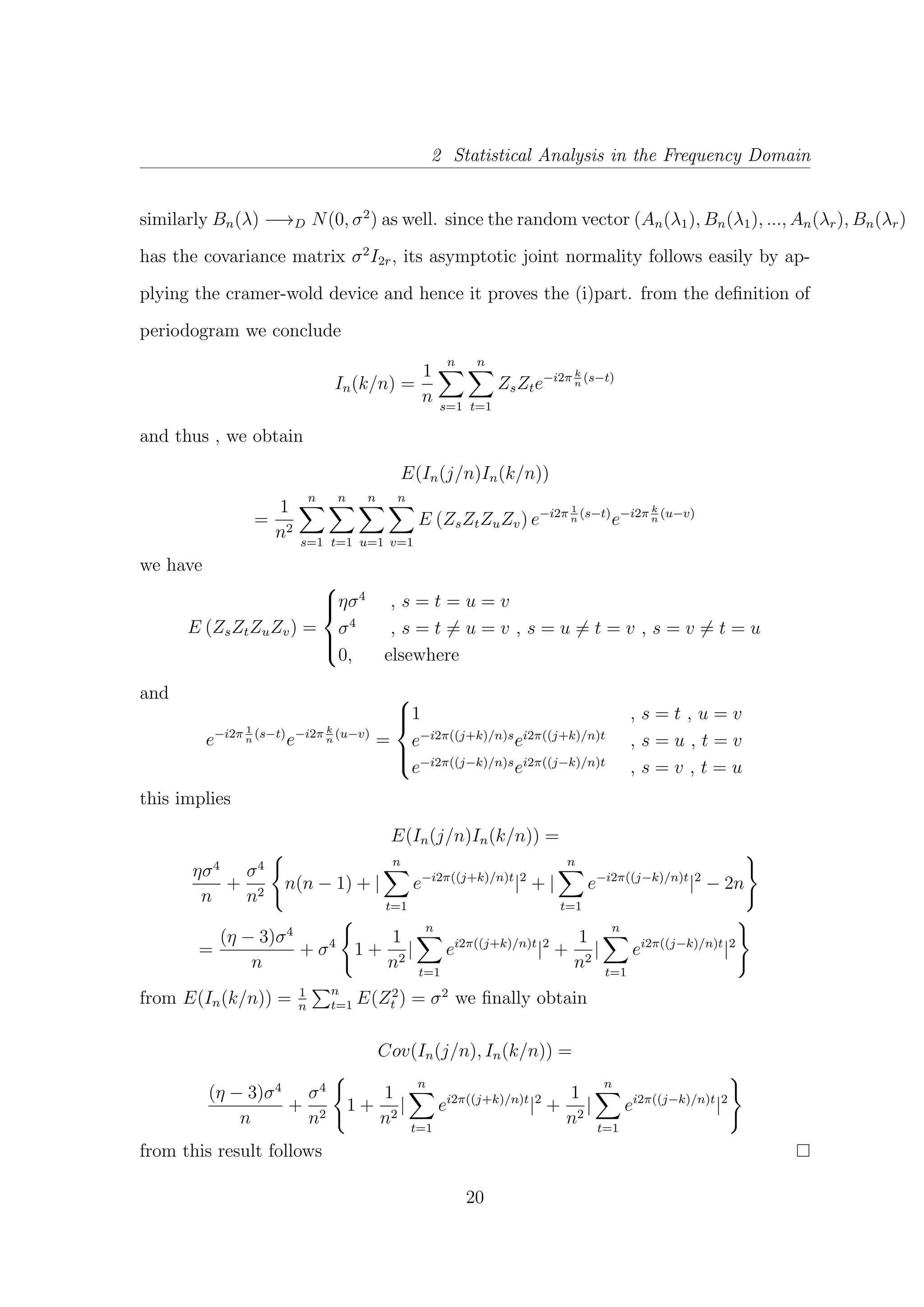
(ii) If E(Z4
t ) = ησ4
< ∞, then we have for k = 0, ..., [n/2] , k ∈ N
V ar(In(k/n)) =
2σ4
+ 1
n
(η − 3)σ4
, k = 0 or k = n/2
σ4
+ 1
n
(η − 3)σ4
elsewhere
and
Cov(In(j/n) , In(k/n)) =
1
n
(η − 3)σ4
, j = k
For N(0, σ2
)-distributed random variables Zt we have η = 3 and, thus, In(k/n) and
In(j/n) are for j = k uncorrelated. we established that they are independent in this
case.
18](https://image.slidesharecdn.com/kavitay1011021-140530015246-phpapp01/75/Time-Series-Analysis-21-2048.jpg)
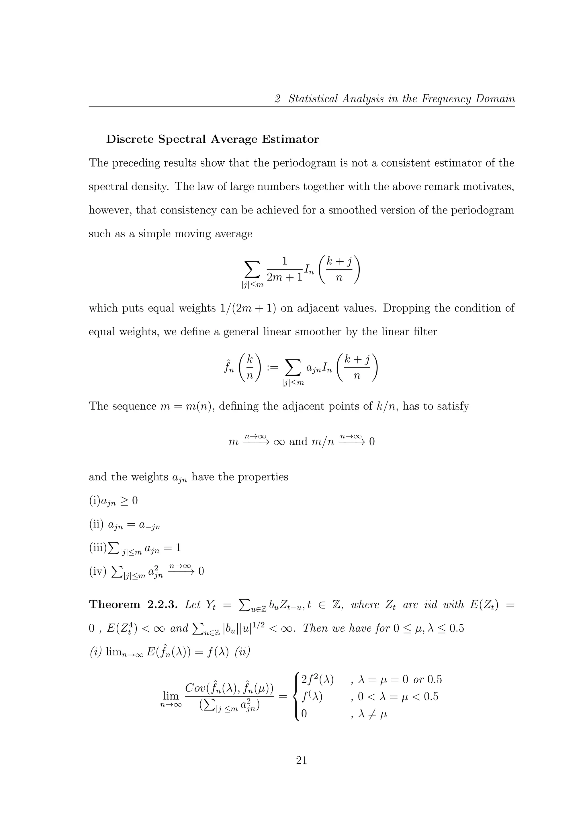
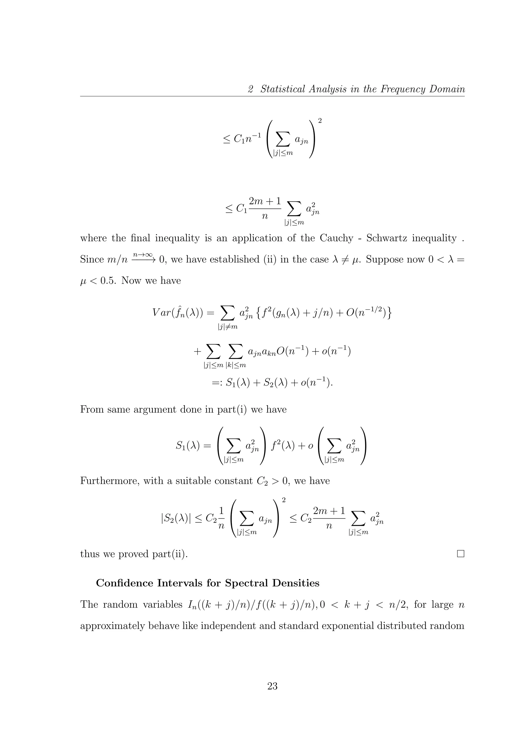
![2 Statistical Analysis in the Frequency Domain
condition (iv) in properties of ajn on weights together with (ii) in the preceding result
entails that V ar( ˆfn(λ))
n→∞
−−−→ 0 for any λ ∈ [0, 0.5]. Together with (i) we, therefore,
obtain that the mean squared error of ˆfn(λ) vanishes asymptotically:
MSE( ˆfn(λ)) = E ( ˆfn(λ) − f(λ))2
= V ar( ˆfn(λ)) + BIAS2
( ˆfn(λ))
n→∞
−−−→ 0
Proof. By the definition of the spectral density estimator we have
|E( ˆfn(λ)) − f(λ)| = |
|j|≤m
ajn {E(In(gn(λ) + j/n)) − f(λ)} |
= |
|j|≤m
ajn {E(In(gn(λ) + j/n)) − f(gn(λ) + j/n) + f(gn(λ) + j/n) − f(λ)} |
where together with the uniform convergence of gn(λ) to λ implies
max
|j|≤m
|gn(λ) + j/n − λ|
n→∞
−−−→ 0
Choose ε > 0. The spectral density f of the process (Yt) is continous and hence we
have
max
|j|≤m
|E(In(gn(λ) + j/n)) − f(gn(λ) + j/n)| < ε/2
if n is large then property (iii) together with triangular inequality implies |E( ˆfn(λ))−
f(λ)| < ε for large n. This implies part from the definition of ˆfn we obtain
Cov( ˆfn(λ), ˆfn(µ))
=
|j|≤m |k|≤m
ajnaknCov (In(gn(λ) + j/n), In(gn(µ) + k/n))
If λ = µ and n sufficiently large we have gn(λ) + j/n = gn(µ) + k/n for arbitrary
|j|, |k| ≤ m. Now there exists a universal constant C1 > 0 such that
|Cov( ˆfn(λ), ˆfn(µ))| = |
|j|≤m |k|≤m
ajnaknO(n−1
)|
22](https://image.slidesharecdn.com/kavitay1011021-140530015246-phpapp01/75/Time-Series-Analysis-25-2048.jpg)
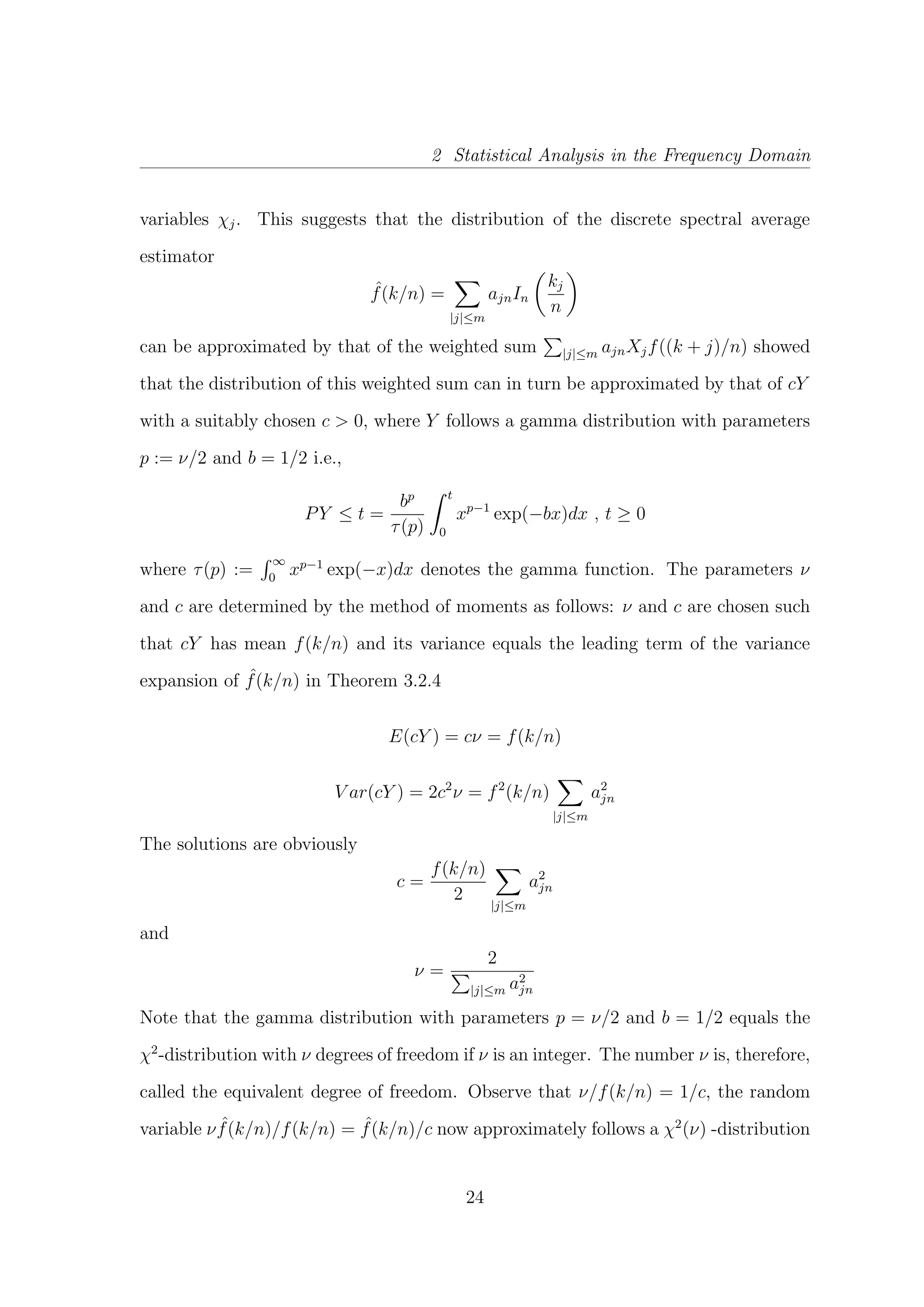
![2 Statistical Analysis in the Frequency Domain
with the convention that χ2
(ν) is the gamma distribution with parameters p = ν/2
and b = 1/2 if ν is not an integer. The interval
ν ˆf(k/n)
χ1−α/2(ν)
,
ν ˆf(k/n)
χ2
α/2
is a confidence interval for f(k/n) of approximate level 1−α , α ∈ (0, 1). By χ2
q(ν) we
denote the q-quantile of the χ2
(ν) -distribution i.e.,P{Y ≤ χ2
q(ν)} = q , 0 < q < 1.
we obtain the confidence interval for log(f(k/n))
Cν,α(k/n) := log( ˆf(k/n)) + log(ν) − log(χ2
1−α/2(ν)) , log( ˆf(k/n)) + log(ν) − log(χ2
α/2(ν))
This interval has constant length log(χ2
1−α/2(ν)/χ2
α/2(ν)). Note that Cν,α(k/n) is
a level (1 − α)-confidence interval only for log(f(λ)) at a fixed Fourier frequency
λ = k/n, with 0 < k < [n/2], but not simultaneously for λ ∈ (0, 0.5).
25](https://image.slidesharecdn.com/kavitay1011021-140530015246-phpapp01/75/Time-Series-Analysis-28-2048.jpg)

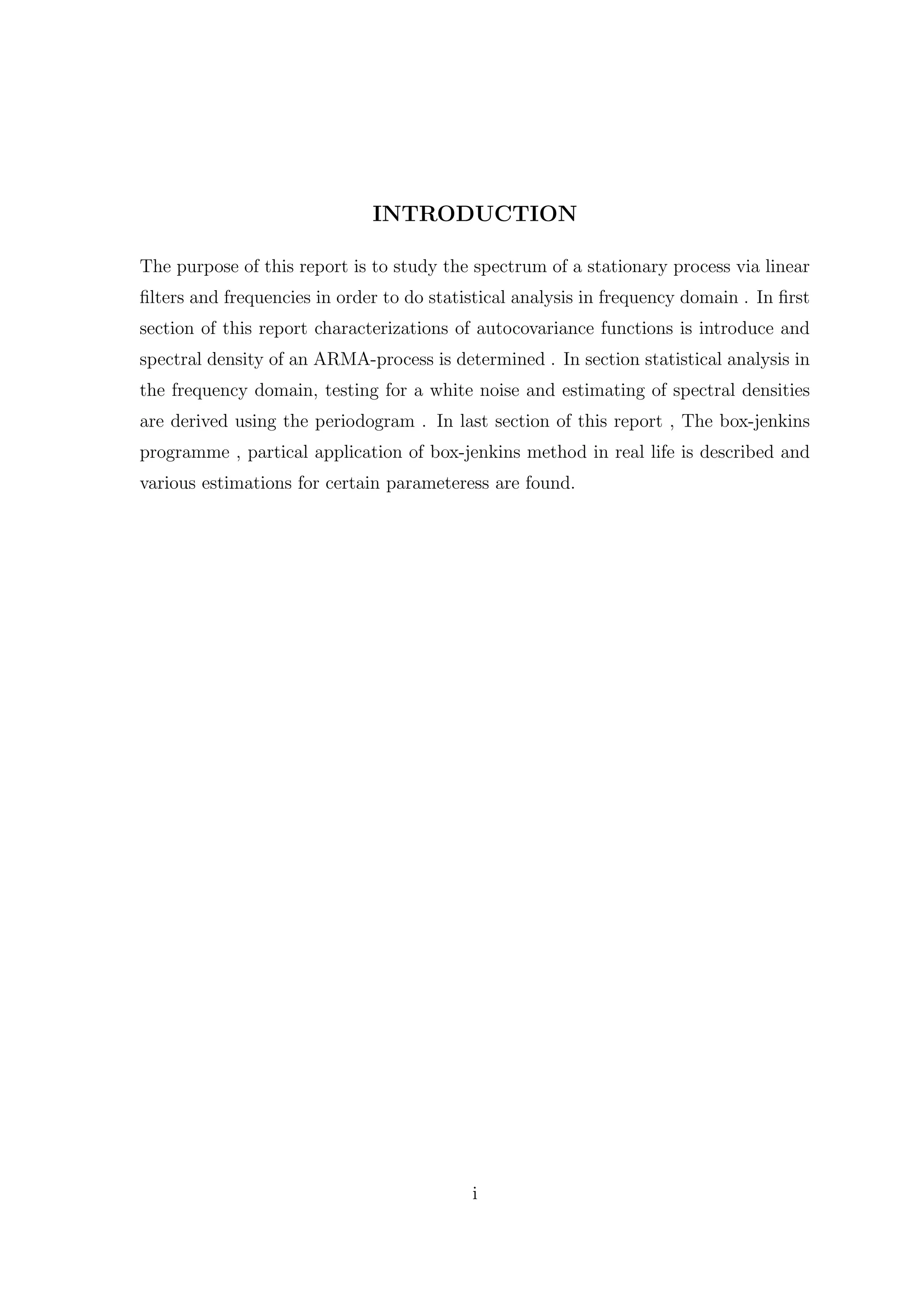
This report, submitted for a Master's degree, focuses on time series analysis of stationary processes through linear filters and frequency domain statistical analysis. It covers autocovariance functions, ARMA process spectral densities, white noise testing, and the Box-Jenkins method application. The report provides detailed mathematical definitions, theorems, and examples related to the spectral density and autocovariance functions.