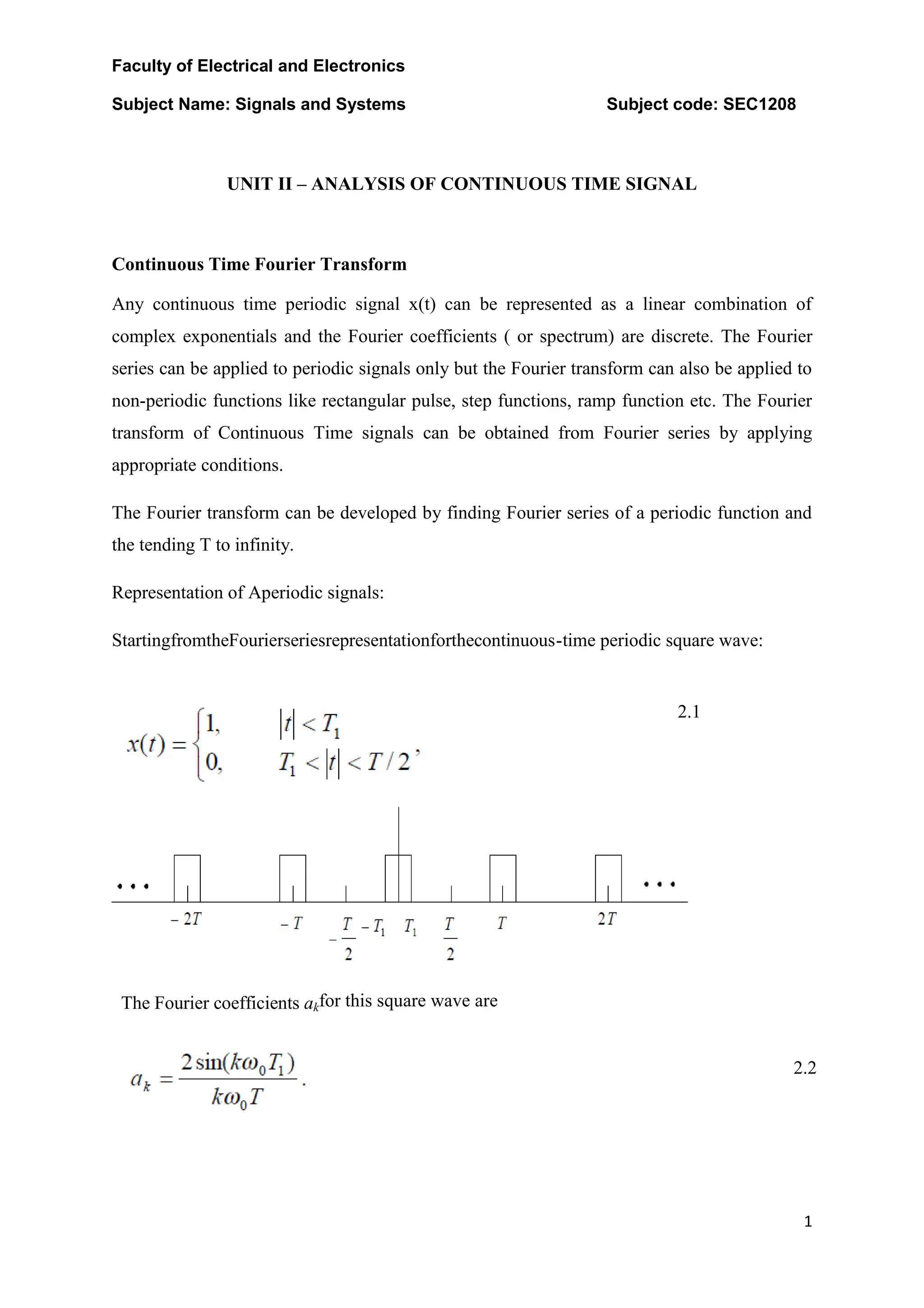
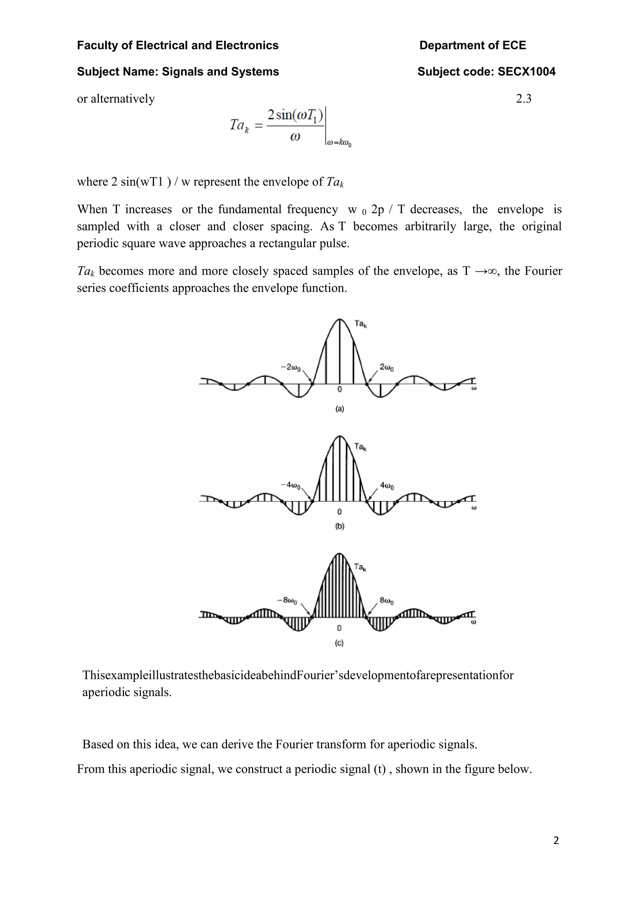
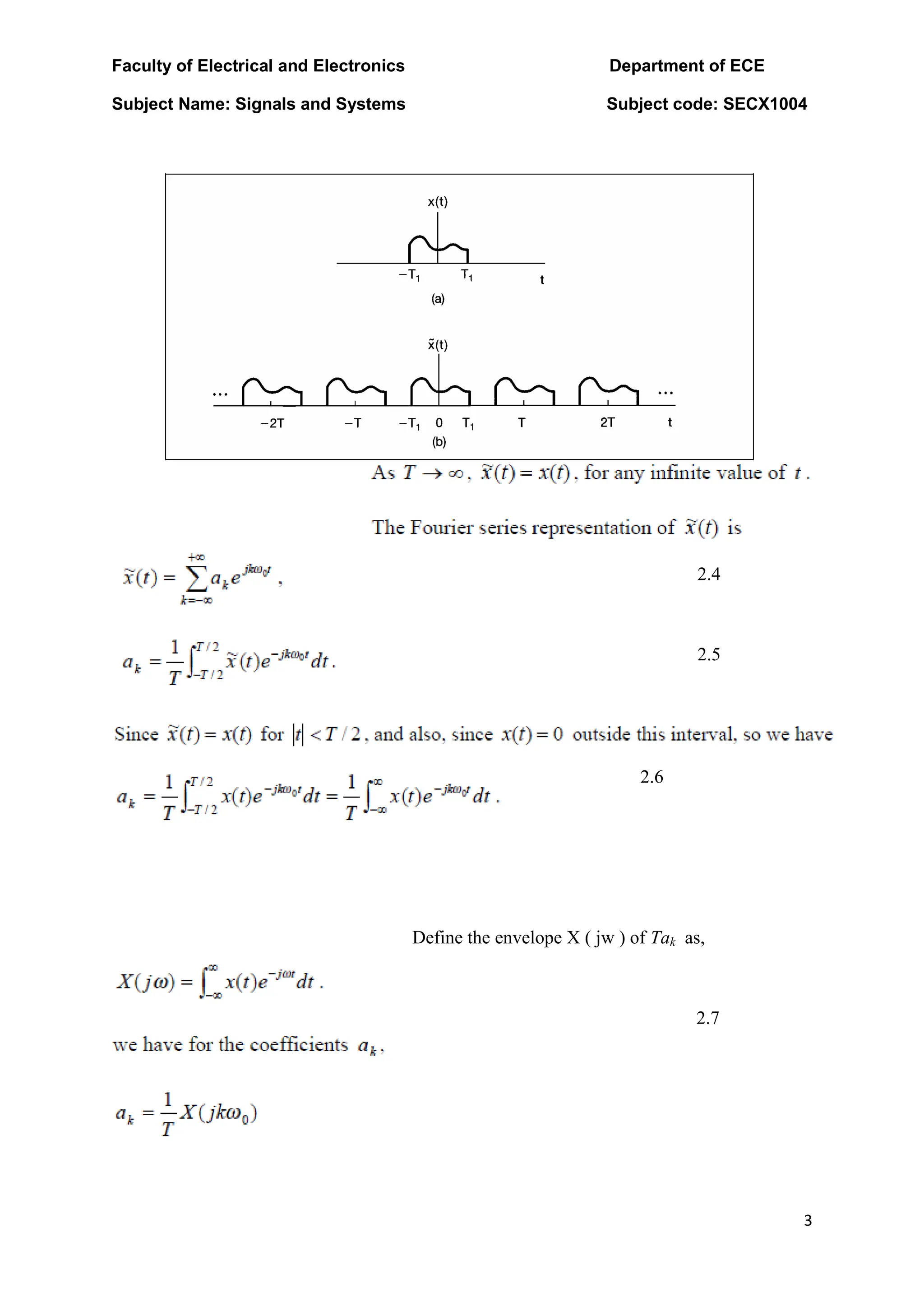
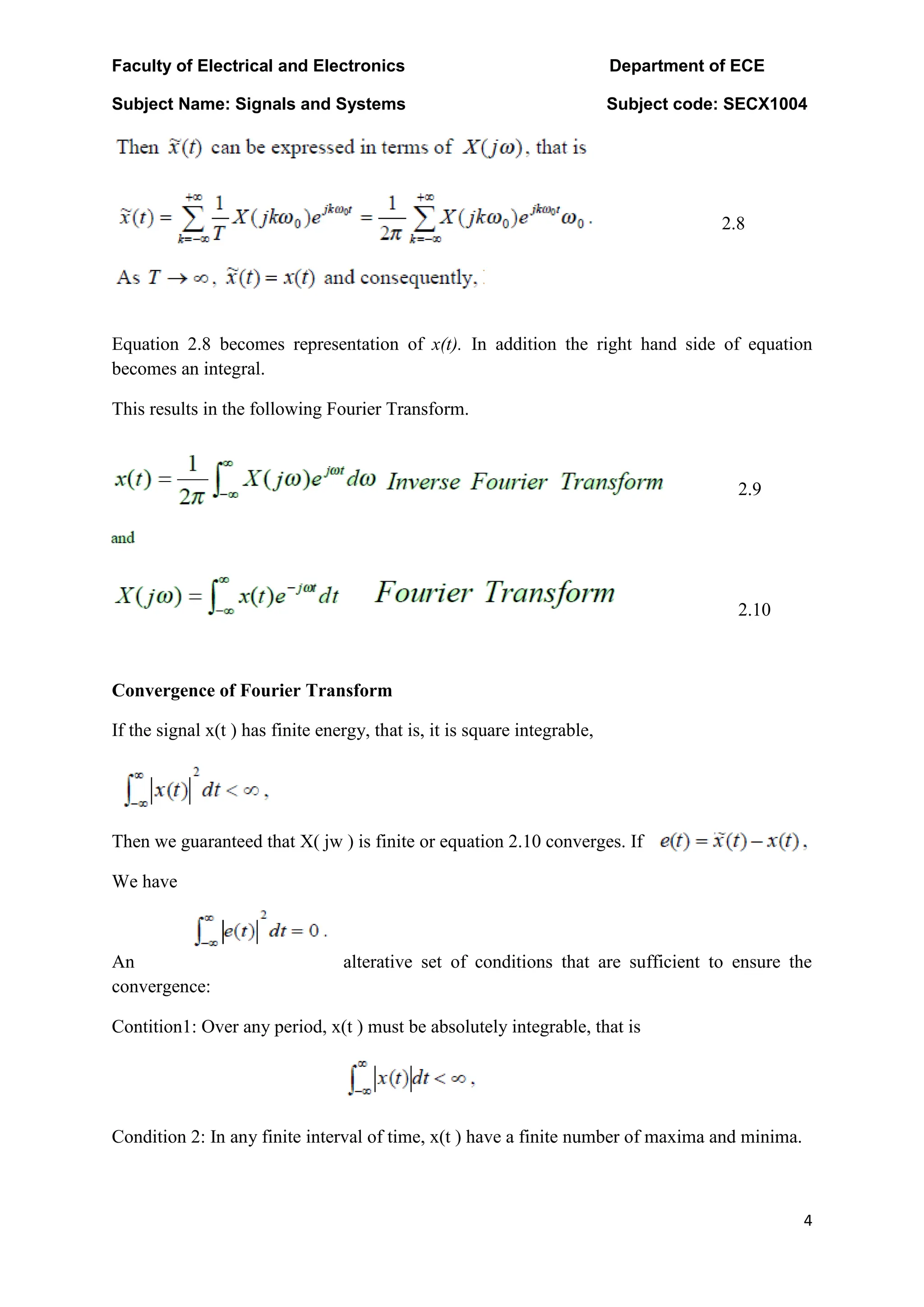
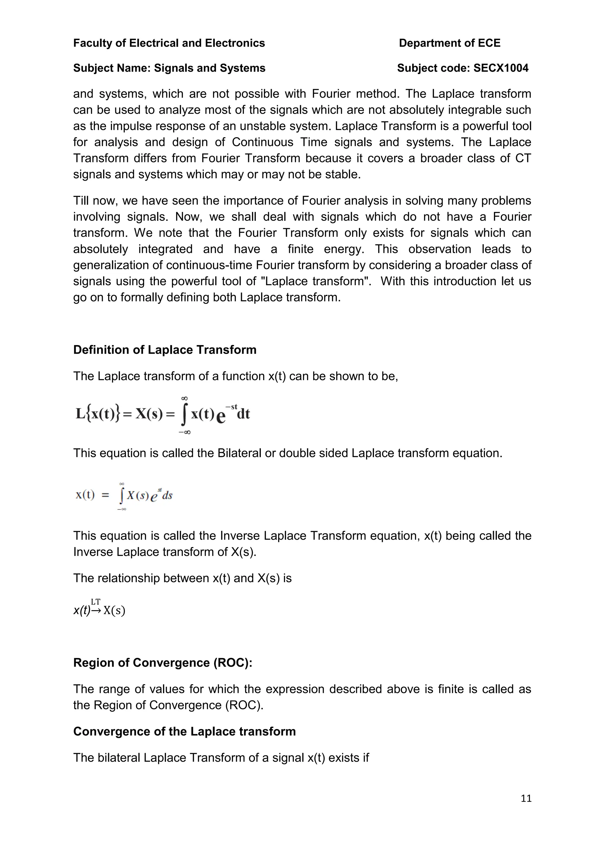
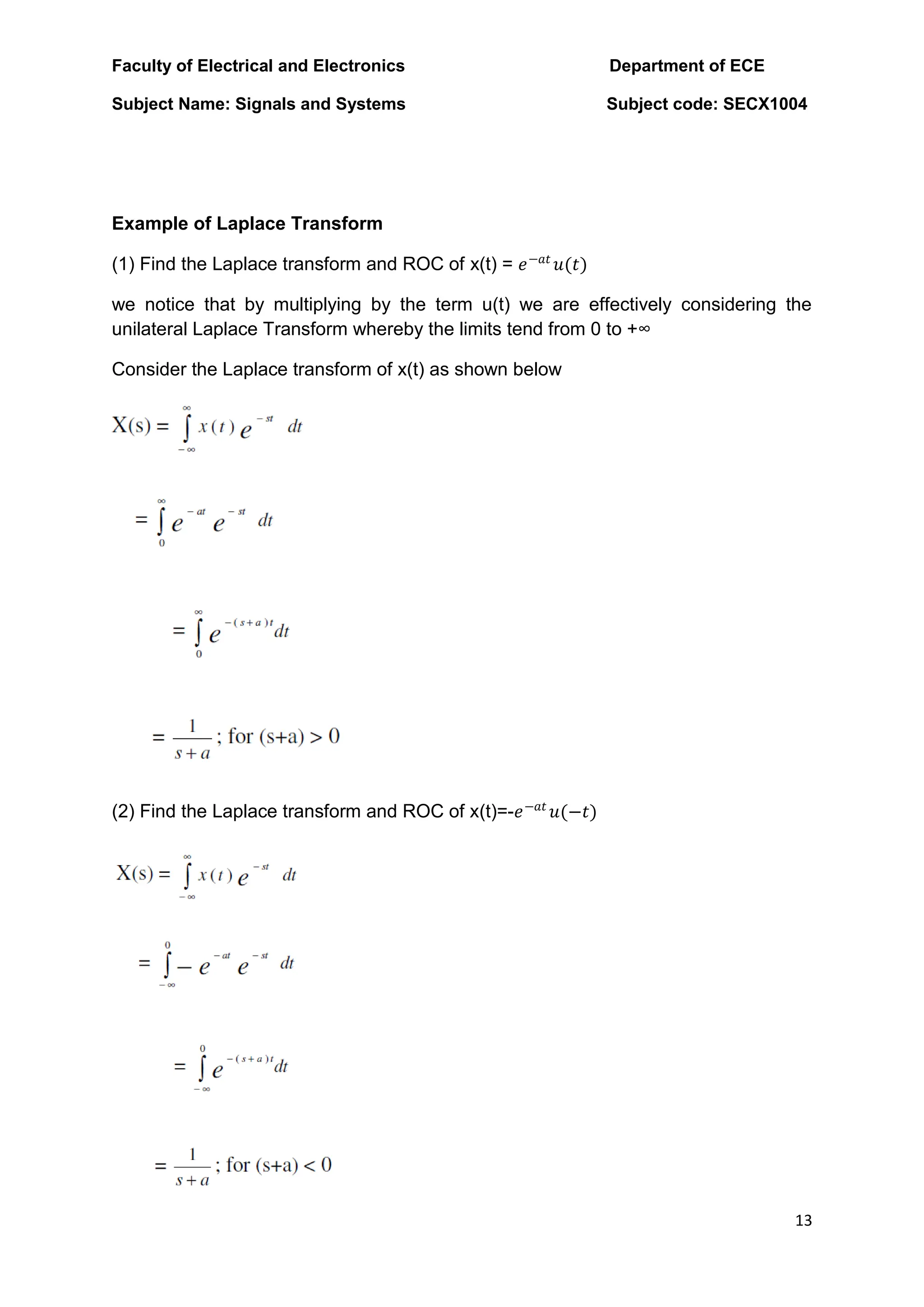
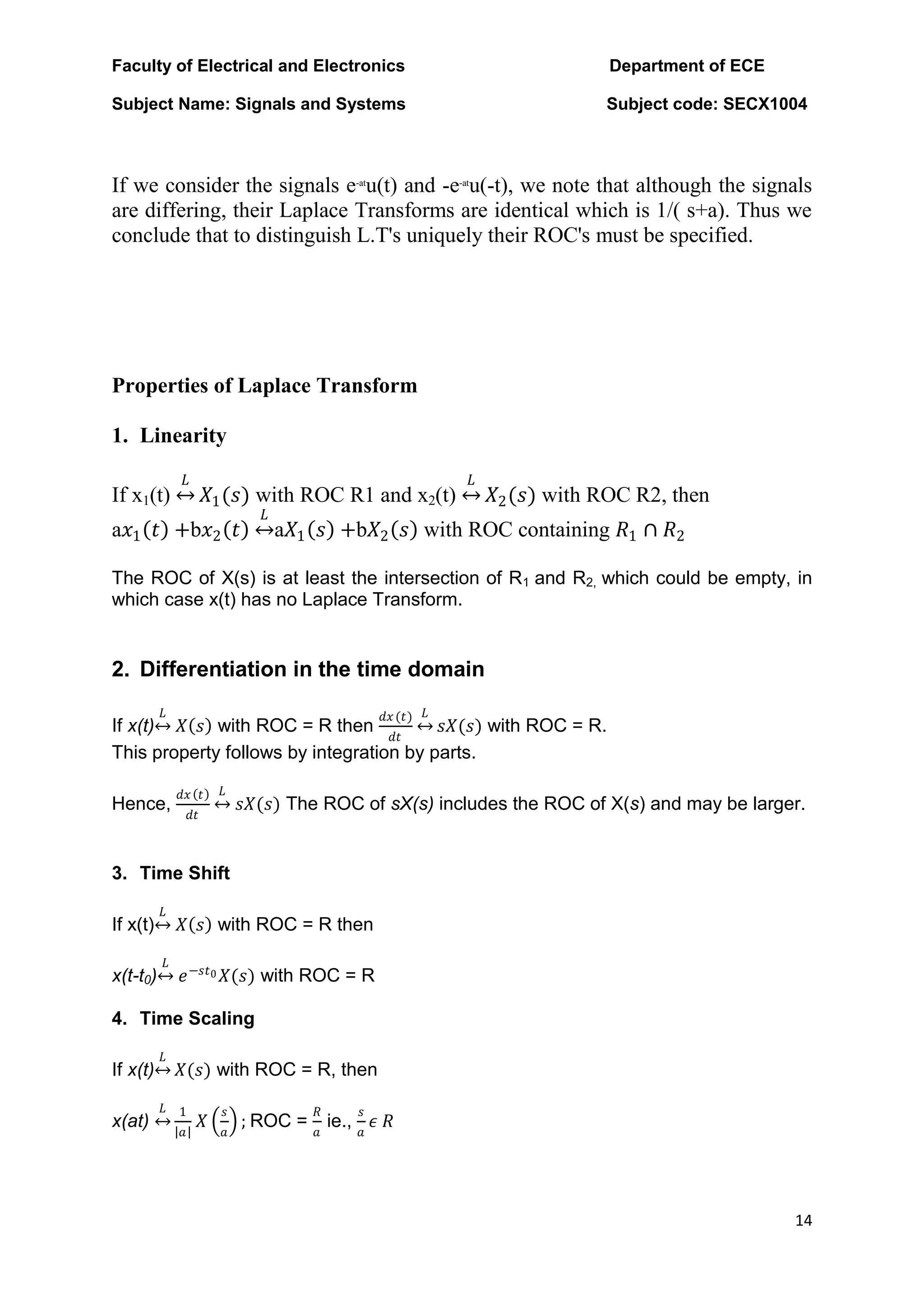
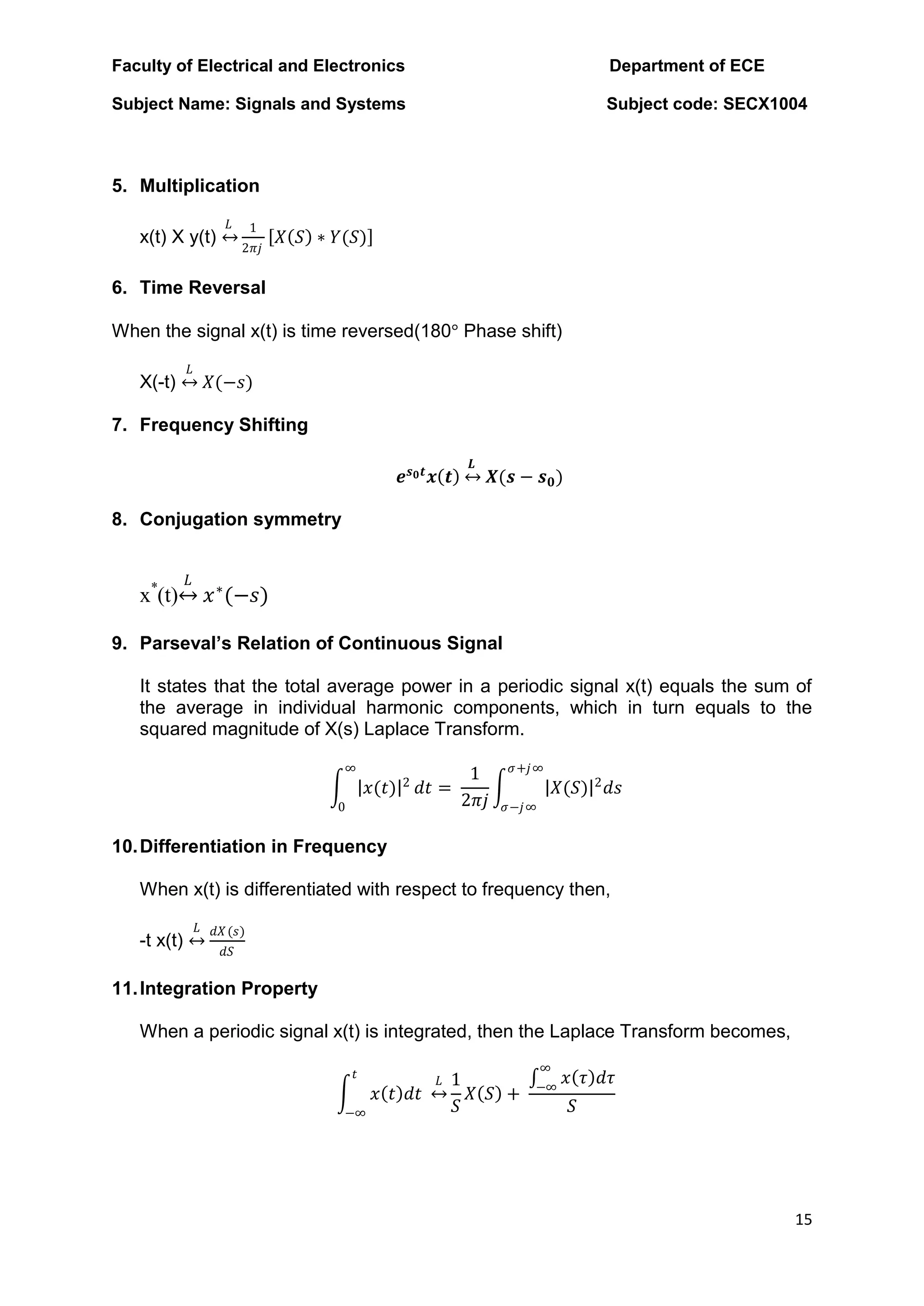
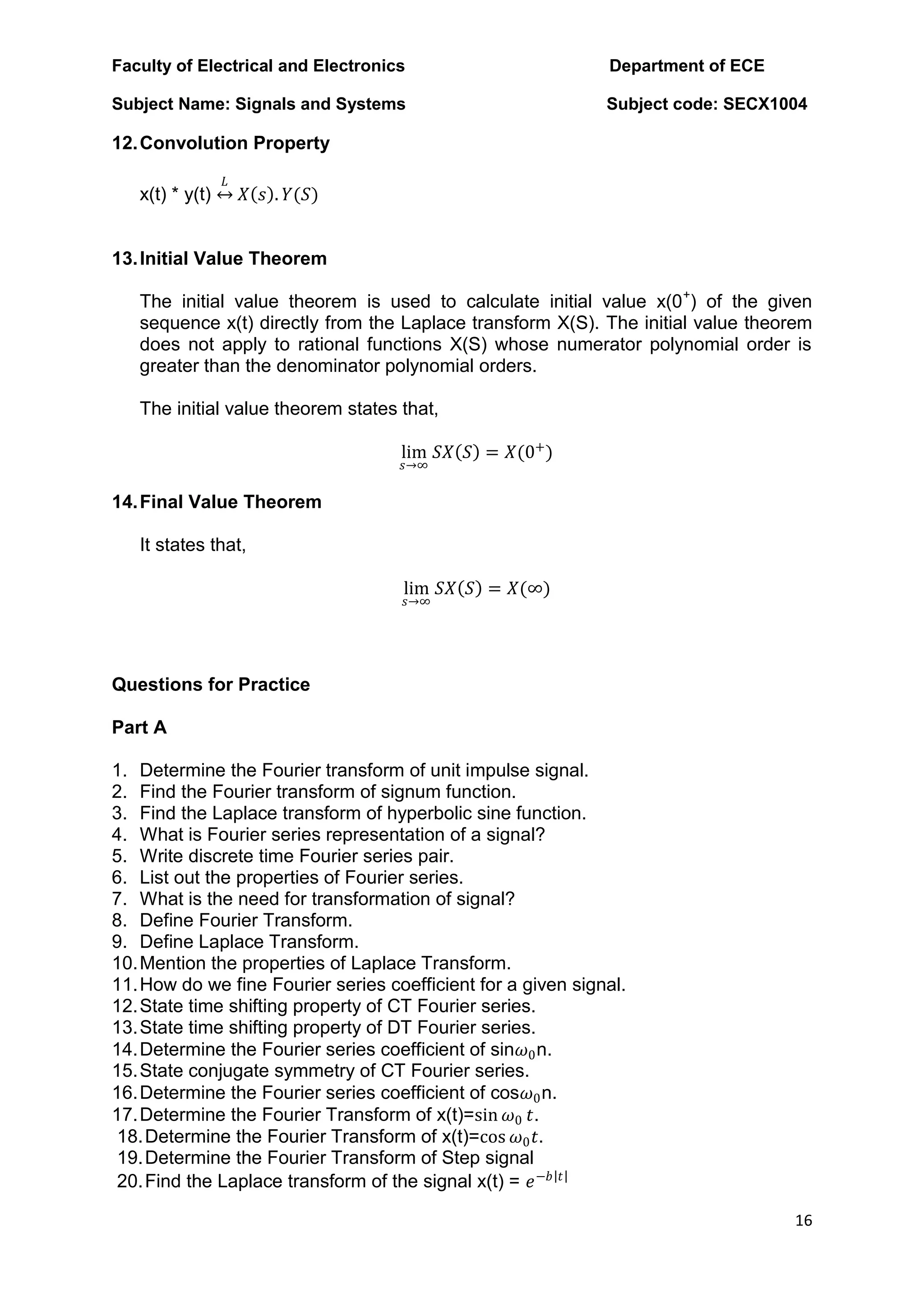
The document discusses the Fourier transform and Laplace transform. Some key points: - The Fourier transform represents periodic and non-periodic signals as a sum of complex exponentials, allowing representation of aperiodic signals. It converges if the signal has finite energy. - The Laplace transform generalizes the Fourier transform to a broader class of signals by using a complex variable 's' instead of just 'jw'. It can represent signals that are not absolutely integrable. 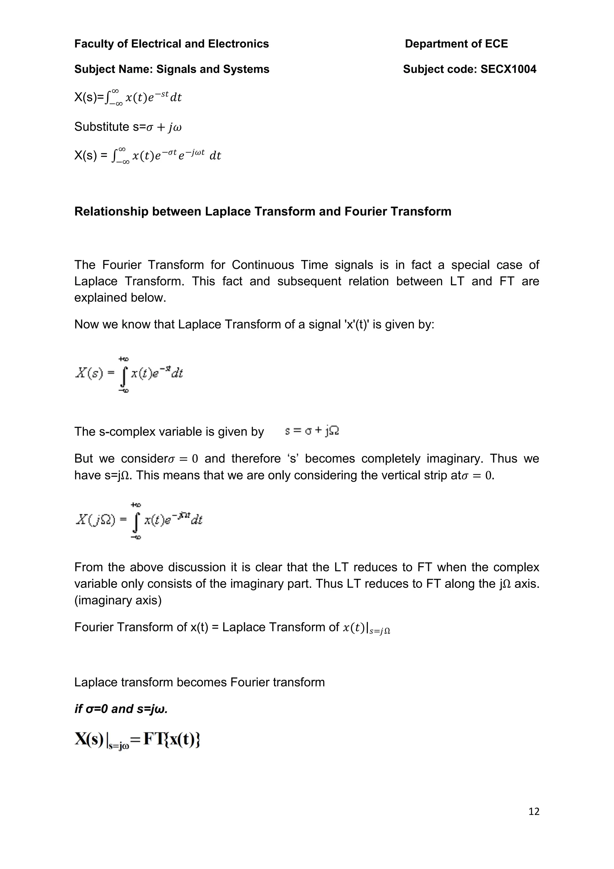- The Fourier transform is a special case of the Laplace transform when s = jw, along the imaginary axis where σ = 0. - Both transforms allow mapping between a signal and its frequency spectrum, with applications in analyzing signals and systems.

1. 1
UNIT II – ANALYSIS OF CONTINUOUS TIME SIGNAL
Continuous Time Fourier Transform
Any continuous time periodic signal x(t) can be represented as a linear combination of
complex exponentials and the Fourier coefficients ( or spectrum) are discrete. The Fourier
series can be applied to periodic signals only but the Fourier transform can also be applied to
non-periodic functions like rectangular pulse, step functions, ramp function etc. The Fourier
transform of Continuous Time signals can be obtained from Fourier series by applying
appropriate conditions.
The Fourier transform can be developed by finding Fourier series of a periodic function and
the tending T to infinity.
Representation of Aperiodic signals:
StartingfromtheFourierseriesrepresentationforthecontinuous-time periodic square wave:
2.1
The Fourier coefficients akfor this square wave are
2.2
Faculty of Electrical and Electronics
Subject Name: Signals and Systems Subject code: SEC1208

2. Faculty of Electrical and Electronics Department of ECE
Subject Name: Signals and Systems Subject code: SECX1004
2
or alternatively 2.3
where 2 sin(wT1 ) / w represent the envelope of Tak
When T increases or the fundamental frequency w 0 2p / T decreases, the envelope is
sampled with a closer and closer spacing. As T becomes arbitrarily large, the original
periodic square wave approaches a rectangular pulse.
Tak becomes more and more closely spaced samples of the envelope, as T →∞, the Fourier
series coefficients approaches the envelope function.
ThisexampleillustratesthebasicideabehindFourier’sdevelopmentofarepresentationfor
aperiodic signals.
Based on this idea, we can derive the Fourier transform for aperiodic signals.
From this aperiodic signal, we construct a periodic signal (t) , shown in the figure below.

3. Faculty of Electrical and Electronics Department of ECE
Subject Name: Signals and Systems Subject code: SECX1004
3
2.4
2.5
2.6
Define the envelope X ( jw ) of Tak as,
2.7

4. Faculty of Electrical and Electronics Department of ECE
Subject Name: Signals and Systems Subject code: SECX1004
4
2.8
Equation 2.8 becomes representation of x(t). In addition the right hand side of equation
becomes an integral.
This results in the following Fourier Transform.
2.9
2.10
Convergence of Fourier Transform
If the signal x(t ) has finite energy, that is, it is square integrable,
Then we guaranteed that X( jw ) is finite or equation 2.10 converges. If
We have
An alterative set of conditions that are sufficient to ensure the
convergence:
Contition1: Over any period, x(t ) must be absolutely integrable, that is
Condition 2: In any finite interval of time, x(t ) have a finite number of maxima and minima.

5. Faculty of Electrical and Electronics Department of ECE
Subject Name: Signals and Systems Subject code: SECX1004
5
Condition 3: In any finite interval of time, there are only a finite number of discontinuities.
Furthermore, each of these discontinuities is finite.
Examples of Continuous-Time Fourier Transform
If a is complex rather than real, we get the same result if Re{a}>0
The Fourier transform can be plotted in terms of the magnitude and phase, as shown in the
figure below.

6. Faculty of Electrical and Electronics Department of ECE
Subject Name: Signals and Systems Subject code: SECX1004
6
Example
Calculate the Fourier transform of the rectangular pulse signal
The inverse Fourier Transform of the sinc function is
Comparing the results we have,
Square wave Sinc Function
This means a square wave in the time domain, its Fourier transform is a sinc function.
However, if the signal in the time domain is a sinc function, then its Fourier transform is a
square wave. This property is referred to as Duality Property.
We also note that when the width of X( jw) increases, its inverse Fourier transform x(t) will
be compressed. When W → ∞, X( jw) converges to an impulse. The transform pair with
several different values of W is shown in the figure below.
FT
FT-1

7. Faculty of Electrical and Electronics Department of ECE
Subject Name: Signals and Systems Subject code: SECX1004
7
The Fourier Transform for Periodic Signals
Properties of Fourier Transform
1. Linearity
If x(t)FX( jw) y(t)FY( jw)
then
ax(t) by(t)FaX ( jw) bY ( jw)
2. Time Shifting
If x(t)FX( jw)
Then
x(t-t0) e-jwt
0 X(jw)
F

8. Faculty of Electrical and Electronics Department of ECE
Subject Name: Signals and Systems Subject code: SECX1004
8
F
F
F
3. Conjugation and Conjugate Symmetry
If x(t) X(jw)
Then
x*
(t) X*
(-jw)
4. Differentiation and Integration
X(jw) then
𝑑𝑥 𝑡
𝑑𝑡
𝐹
𝑗𝜔𝑋(𝑗𝜔)
If x(t)
𝑥 𝜏 𝑑𝜏
𝑡
−∞
𝐹 1
𝑗𝜔
𝑋 𝑗𝑤 + 𝜋𝑋 0 𝛿 𝜔
5. Time and Frequency Scaling
x(t)
𝐹
𝑋(𝑗𝜔)
then,
x(at)
𝐹 1
𝑎
𝑋
𝑗𝜔
𝑎
From the equation we see that the signal is compressed in the time domain, the
spectrum will be extended in the frequency domain. Conversely, if the signal is
extended, the corresponding spectrum will be compressed.
If a = -1, we get from the above equation,
X(-t)
𝐹
𝑋(𝑗𝜔)
That is reversing a signal in time also reverses its Fourier transform.
6. Duality
The duality of the Fourier Transform can be demonstrated using the following
example.
x1(t)=
1, 𝑡 < 𝑇1
0, 𝑡 > 𝑇1
𝐹
𝑋1
(𝑗𝜔 )
=
2 sin 𝜔𝑇1
𝜔

9. Faculty of Electrical and Electronics Department of ECE
Subject Name: Signals and Systems Subject code: SECX1004
9
x2(t) =
𝑠𝑖𝑛𝑊 𝑇1
𝜋𝑡
𝐹
𝑋2 𝑗𝜔 =
1, 𝜔 < 𝑊
0, 𝜔 > 𝑊
For any transform pair, there is a dual pair with the time and frequency variables
interchanged.
Parseval’s Relation
If x(t)
𝐹
𝑋(𝑗𝜔),
We have,
𝑥(𝑡) 2
𝑑𝑡 =
1
2𝜋
∞
−∞
𝑋(𝑗𝑤) 2
∞
−∞
𝑑𝜔
Parseval‟s relation states that the total energy may be determined either by
computing the energy per unit time 𝑥(𝑡) 2
and integrating over all time or by
computing the energy per unit frequency 𝑥(𝑗𝜔) 2
2𝜋 and integrating over all

10. Faculty of Electrical and Electronics Department of ECE
Subject Name: Signals and Systems Subject code: SECX1004
10
frequencies. For this reason, 𝑥(𝑗𝜔) 2
is often referred toas the energy density
spectrum.
The Parseval's theorem states that the inner product between signals is preserved in
going from time to the frequency domain. This is interpreted physically as “Energy
calculated in the time domain is sameas the energy calculated in the frequency
domain”
The convolution properties
𝑦 𝑡 = ℎ 𝑡 ∗ 𝒙 𝑡
𝑭
𝑌 𝑗𝜔 = 𝐻 𝑗𝜔 𝑋(𝑗𝜔)
The equation shows that the Fourier transform maps the convolution of two signals into
product of their Fourier transforms.
H(j𝜔), the transform of the impulse response is the frequency response of the LTI system,
which also completely characterizes an LTI system.
Example
The frequency response of a differentiator.
y(t)=
𝑑𝑥(𝑡)
𝑑𝑡
From the differentiation property,
Y(j𝜔)= j𝜔𝑋 𝑗𝜔
The frequency response of the differentiator is,
H(j𝜔)=
𝑌(𝑗𝜔 )
𝑋(𝑗𝜔 )
=j𝜔
The Multiplication Property
Multiplication of one signal by another can be thought of as one signal to scale or modulate
the amplitude of the other, and consequently, the multiplication of two signals is often
referred to as amplitude modulation.
Laplace Transform
The Laplace Transform is the more generalized representation of CT complex
exponential signals. The Laplace transform provide solutions to most of the signals

11. Faculty of Electrical and Electronics Department of ECE
Subject Name: Signals and Systems Subject code: SECX1004
11
and systems, which are not possible with Fourier method. The Laplace transform
can be used to analyze most of the signals which are not absolutely integrable such
as the impulse response of an unstable system. Laplace Transform is a powerful tool
for analysis and design of Continuous Time signals and systems. The Laplace
Transform differs from Fourier Transform because it covers a broader class of CT
signals and systems which may or may not be stable.
Till now, we have seen the importance of Fourier analysis in solving many problems
involving signals. Now, we shall deal with signals which do not have a Fourier
transform. We note that the Fourier Transform only exists for signals which can
absolutely integrated and have a finite energy. This observation leads to
generalization of continuous-time Fourier transform by considering a broader class of
signals using the powerful tool of "Laplace transform". With this introduction let us
go on to formally defining both Laplace transform.
Definition of Laplace Transform
The Laplace transform of a function x(t) can be shown to be,
This equation is called the Bilateral or double sided Laplace transform equation.
This equation is called the Inverse Laplace Transform equation, x(t) being called the
Inverse Laplace transform of X(s).
The relationship between x(t) and X(s) is
x(t)
LT
X(s)
Region of Convergence (ROC):
The range of values for which the expression described above is finite is called as
the Region of Convergence (ROC).
Convergence of the Laplace transform
The bilateral Laplace Transform of a signal x(t) exists if

12. Faculty of Electrical and Electronics Department of ECE
Subject Name: Signals and Systems Subject code: SECX1004
12
X(s)= 𝑥(𝑡)𝑒−𝑠𝑡
𝑑𝑡
∞
−∞
Substitute s=𝜎 + 𝑗𝜔
X(s) = 𝑥(𝑡)𝑒−𝜎𝑡
𝑒−𝑗𝜔𝑡
∞
−∞
𝑑𝑡
Relationship between Laplace Transform and Fourier Transform
The Fourier Transform for Continuous Time signals is in fact a special case of
Laplace Transform. This fact and subsequent relation between LT and FT are
explained below.
Now we know that Laplace Transform of a signal 'x'(t)' is given by:
The s-complex variable is given by
But we consider𝜎 = 0 and therefore „s‟ becomes completely imaginary. Thus we
have s=jΩ. This means that we are only considering the vertical strip at𝜎 = 0.
From the above discussion it is clear that the LT reduces to FT when the complex
variable only consists of the imaginary part. Thus LT reduces to FT along the jΩ axis.
(imaginary axis)
Fourier Transform of x(t) = Laplace Transform of 𝑥(𝑡) 𝑠=𝑗Ω
Laplace transform becomes Fourier transform
if σ=0 and s=jω.

13. Faculty of Electrical and Electronics Department of ECE
Subject Name: Signals and Systems Subject code: SECX1004
13
Example of Laplace Transform
(1) Find the Laplace transform and ROC of x(t) = 𝑒−𝑎𝑡
𝑢(𝑡)
we notice that by multiplying by the term u(t) we are effectively considering the
unilateral Laplace Transform whereby the limits tend from 0 to +∞
Consider the Laplace transform of x(t) as shown below
(2) Find the Laplace transform and ROC of x(t)=-𝑒−𝑎𝑡
𝑢(−𝑡)

14. Faculty of Electrical and Electronics Department of ECE
Subject Name: Signals and Systems Subject code: SECX1004
14
If we consider the signals e-at
u(t) and -e-at
u(-t), we note that although the signals
are differing, their Laplace Transforms are identical which is 1/( s+a). Thus we
conclude that to distinguish L.T's uniquely their ROC's must be specified.
Properties of Laplace Transform
1. Linearity
If x1(t)
𝐿
𝑋1(𝑠) with ROC R1 and x2(t)
𝐿
𝑋2(𝑠) with ROC R2, then
a𝑥1 𝑡 +b𝑥2 𝑡
𝐿
a𝑋1 𝑠 +b𝑋2 𝑠 with ROC containing 𝑅1 ∩ 𝑅2
The ROC of X(s) is at least the intersection of R1 and R2, which could be empty, in
which case x(t) has no Laplace Transform.
2. Differentiation in the time domain
If x(t)
𝐿
𝑋 𝑠 with ROC = R then
𝑑𝑥(𝑡)
𝑑𝑡
𝐿
𝑠𝑋(𝑠) with ROC = R.
This property follows by integration by parts.
Hence,
𝑑𝑥 𝑡
𝑑𝑡
𝐿
𝑠𝑋(𝑠) The ROC of sX(s) includes the ROC of X(s) and may be larger.
3. Time Shift
If x(t)
𝐿
𝑋 𝑠 with ROC = R then
x(t-t0)
𝐿
𝑒−𝑠𝑡0 𝑋(𝑠) with ROC = R
4. Time Scaling
If x(t)
𝐿
𝑋(𝑠) with ROC = R, then
x(at)
𝐿 1
𝑎
𝑋
𝑠
𝑎
; ROC =
𝑅
𝑎
ie.,
𝑠
𝑎
𝜖 𝑅

15. Faculty of Electrical and Electronics Department of ECE
Subject Name: Signals and Systems Subject code: SECX1004
15
5. Multiplication
x(t) X y(t)
𝐿 1
2𝜋𝑗
𝑋 𝑆 ∗ 𝑌(𝑆)
6. Time Reversal
When the signal x(t) is time reversed(180° Phase shift)
X(-t)
𝐿
𝑋(−𝑠)
7. Frequency Shifting
𝒆𝒔𝟎𝒕
𝒙 𝒕
𝑳
𝑿(𝒔 − 𝒔𝟎)
8. Conjugation symmetry
x*
(t)
𝐿
𝑥∗
(−𝑠)
9. Parseval’s Relation of Continuous Signal
It states that the total average power in a periodic signal x(t) equals the sum of
the average in individual harmonic components, which in turn equals to the
squared magnitude of X(s) Laplace Transform.
𝑥(𝑡) 2
∞
0
𝑑𝑡 =
1
2𝜋𝑗
𝑋(𝑆) 2
𝑑𝑠
𝜎+𝑗∞
𝜎−𝑗∞
10.Differentiation in Frequency
When x(t) is differentiated with respect to frequency then,
-t x(t)
𝐿 𝑑𝑋(𝑠)
𝑑𝑆
11.Integration Property
When a periodic signal x(t) is integrated, then the Laplace Transform becomes,
𝑥 𝑡 𝑑𝑡
𝐿
𝑡
−∞
1
𝑆
𝑋 𝑆 +
𝑥 𝜏 𝑑𝜏
∞
−∞
𝑆

16. Faculty of Electrical and Electronics Department of ECE
Subject Name: Signals and Systems Subject code: SECX1004
16
12.Convolution Property
x(t) * y(t)
𝐿
𝑋 𝑠 . 𝑌(𝑆)
13.Initial Value Theorem
The initial value theorem is used to calculate initial value x(0+
) of the given
sequence x(t) directly from the Laplace transform X(S). The initial value theorem
does not apply to rational functions X(S) whose numerator polynomial order is
greater than the denominator polynomial orders.
The initial value theorem states that,
lim
𝑠→∞
𝑆𝑋 𝑆 = 𝑋(0+
)
14.Final Value Theorem
It states that,
lim
𝑠→∞
𝑆𝑋 𝑆 = 𝑋(∞)
Questions for Practice
Part A
1. Determine the Fourier transform of unit impulse signal.
2. Find the Fourier transform of signum function.
3. Find the Laplace transform of hyperbolic sine function.
4. What is Fourier series representation of a signal?
5. Write discrete time Fourier series pair.
6. List out the properties of Fourier series.
7. What is the need for transformation of signal?
8. Define Fourier Transform.
9. Define Laplace Transform.
10.Mention the properties of Laplace Transform.
11.How do we fine Fourier series coefficient for a given signal.
12.State time shifting property of CT Fourier series.
13.State time shifting property of DT Fourier series.
14.Determine the Fourier series coefficient of sin𝜔0n.
15.State conjugate symmetry of CT Fourier series.
16.Determine the Fourier series coefficient of cos𝜔0n.
17.Determine the Fourier Transform of x(t)=sin 𝜔0 𝑡.
18.Determine the Fourier Transform of x(t)=cos 𝜔0𝑡.
19.Determine the Fourier Transform of Step signal
20.Find the Laplace transform of the signal x(t) = 𝑒−𝑏 𝑡

17. Faculty of Electrical and Electronics Department of ECE
Subject Name: Signals and Systems Subject code: SECX1004
17
Part B
1. State Parseval‟s theorem for discrete time signal.
2. Find the FT of the following and sketch the magnitude and phase spectrum
(i) x(t) = 𝛿(𝑡)
(ii) x(t) = 𝑒−𝑎𝑡
𝑢(𝑡)
(iii) x(t) = 𝑒−𝑡
(iv) x(t) = 𝑒2𝑡
𝑢 𝑡
3. Find the Laplace transform of
(i) x(t) = 𝛿 𝑡
(ii) x(t) = u(t)
(iii) x(t) = cos Ω0 𝑡
(iv) x(t) = sin 𝜔𝑡𝑢(𝑡)
4. Determine initial and final value of a signal x(t) = sin 2𝑡 𝑢(𝑡)
5. Determine the initial and final value of signal x(t) whose unilateral Laplace
Transform is,
X(S) =
2𝑠+5
𝑠(𝑠+3)
6. State and prove the properties of Fourier Transform.
7. State and prove the properties of Laplace Transform.