Download to read offline


![Problem 5:
(a) s − 3
H(s) = K
s + 3
�
|H (j Ω
)| = |K |�
�
�
j Ω− 3� �
= |K |
�
j Ω+ 3�
(b) Consider this pole-zero plot:
j
s -p I a
n
r
r
r
1 q
q
2
q
3
Let the vectors from the poles and zeros to an arbitrary test frequency Ωbe ri and qi:
|H (j Ω
)| = |K |
|q1||q2||q3|
= |K |
|r1||r1||r1|
since |qi| = |ri| for all i regardless of the system order. Therefore, this given pole-zero configuration, as well as all who
satisfy problem conditions, are all-pass filters.
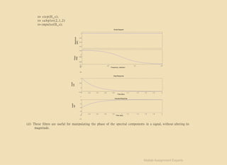
(c) M AT LA B C om m and − line :
>> H_s=tf([1 -3], [1 3])
Transfer function: s - 3
s + 3
>> bode(H_s);
>> subplot(2,1,1)
Matlab Assignment Experts](https://image.slidesharecdn.com/matlabassignmentexperts-211009074042/85/Signal-Processing-Homework-Help-10-320.jpg)

The document discusses various problems related to signal processing, including waveforms, filtering, and the Gibbs phenomenon in Fourier analysis. It outlines assignments that require working with MATLAB to analyze filter responses, impulse responses, and the effects of truncating Fourier series on waveforms. The document emphasizes understanding the mathematical principles behind these concepts and their practical implications in signal processing.