Downloaded 453 times


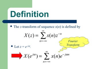

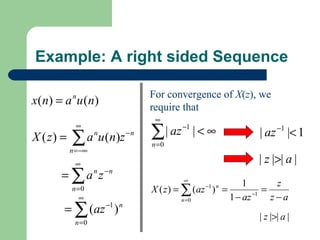

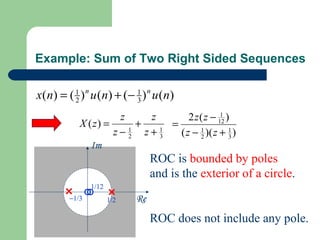

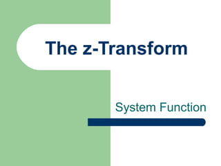
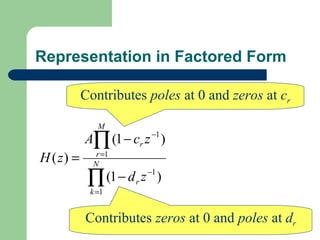
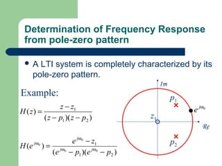
![Z-Transform Pairs
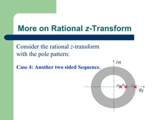
Sequence z-Transform ROC
1 − [cos ω0 ] z −1
[cos ω0 n]u (n) | z |> 1
1 − [ 2 cos ω0 ]z −1 + z −2
[sin ω0 ]z −1
[sin ω0 n]u (n) | z |> 1
1 − [2 cos ω0 ]z −1 + z −2
1 − [ r cos ω0 ]z −1
[r n cos ω0 n]u (n) | z |> r
1 − [ 2r cos ω0 ]z −1 + r 2 z − 2
[r sin ω0 ] z −1
[r n sin ω0 n]u (n) | z |> r
1 − [ 2r cos ω0 ]z −1 + r 2 z − 2
a n 0 ≤ n ≤ N −1 1− aN z−N
| z |> 0
0 otherwise 1 − az −1](https://image.slidesharecdn.com/z-transformroc-121116092757-phpapp01/85/Z-transform-ROC-eng-Math-35-320.jpg)

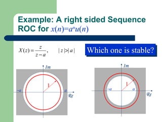
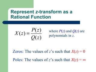
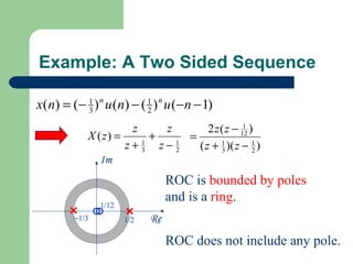
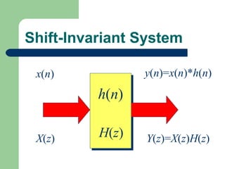
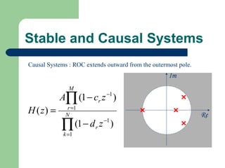
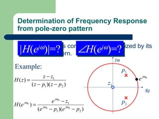
![Linearity
Z [ x(n)] = X ( z ), z ∈ Rx
Z [ y (n)] = Y ( z ), z ∈ Ry
Z [ax(n) + by (n)] = aX ( z ) + bY ( z ), z ∈ Rx ∩ R y
Overlay of
the above two
ROC’s](https://image.slidesharecdn.com/z-transformroc-121116092757-phpapp01/85/Z-transform-ROC-eng-Math-38-320.jpg)
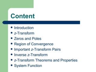
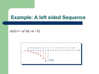
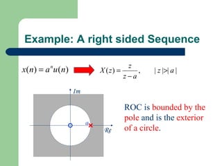
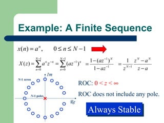
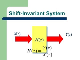
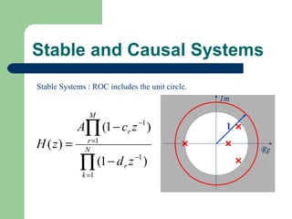
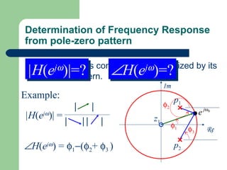
![Shift
Z [ x(n)] = X ( z ), z ∈ Rx
Z [ x(n + n0 )] = z X ( z )
n0
z ∈ Rx](https://image.slidesharecdn.com/z-transformroc-121116092757-phpapp01/85/Z-transform-ROC-eng-Math-39-320.jpg)
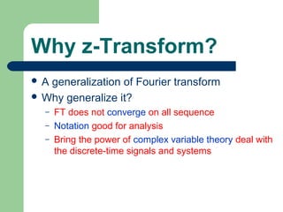
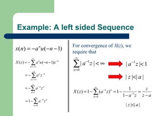
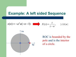
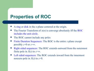
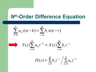
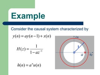
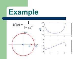
![Multiplication by an Exponential Sequence
Z [ x(n)] = X ( z ), Rx- <| z |< Rx +
−1
Z [a x(n)] = X (a z )
n
z ∈| a | ⋅Rx](https://image.slidesharecdn.com/z-transformroc-121116092757-phpapp01/85/Z-transform-ROC-eng-Math-40-320.jpg)
![Differentiation of X(z)
Z [ x(n)] = X ( z ), z ∈ Rx
dX ( z )
Z [nx(n)] = − z z ∈ Rx
dz](https://image.slidesharecdn.com/z-transformroc-121116092757-phpapp01/85/Z-transform-ROC-eng-Math-41-320.jpg)
![Conjugation
Z [ x(n)] = X ( z ), z ∈ Rx
Z [ x * (n)] = X * ( z*) z ∈ Rx](https://image.slidesharecdn.com/z-transformroc-121116092757-phpapp01/85/Z-transform-ROC-eng-Math-42-320.jpg)
![Reversal
Z [ x(n)] = X ( z ), z ∈ Rx
−1
Z [ x(−n)] = X ( z ) z ∈ 1 / Rx](https://image.slidesharecdn.com/z-transformroc-121116092757-phpapp01/85/Z-transform-ROC-eng-Math-43-320.jpg)
![Real and Imaginary Parts
Z [ x(n)] = X ( z ), z ∈ Rx
Re[ x(n)] = 1 [ X ( z ) + X * ( z*)]
2 z ∈ Rx
Im[ x(n)] = 1
2j [ X ( z ) − X * ( z*)] z ∈ Rx](https://image.slidesharecdn.com/z-transformroc-121116092757-phpapp01/85/Z-transform-ROC-eng-Math-44-320.jpg)
![Convolution of Sequences
Z [ x(n)] = X ( z ), z ∈ Rx
Z [ y (n)] = Y ( z ), z ∈ Ry
Z [ x(n) * y (n)] = X ( z )Y ( z ) z ∈ Rx ∩ R y](https://image.slidesharecdn.com/z-transformroc-121116092757-phpapp01/85/Z-transform-ROC-eng-Math-46-320.jpg)
![Convolution of Sequences
∞
x ( n) * y ( n) = ∑ x(k ) y (n − k )
k = −∞
∞
∞
−n
Z [ x(n) * y (n)] = ∑ ∑ x(k ) y (n − k ) z
n = −∞ k = −∞
∞ ∞ ∞ ∞
= ∑ x(k ) ∑ y(n − k )z −n
= ∑
k = −∞
x(k ) z − k ∑ y (n)z − n
n = −∞
k = −∞ n = −∞
= X ( z )Y ( z )](https://image.slidesharecdn.com/z-transformroc-121116092757-phpapp01/85/Z-transform-ROC-eng-Math-47-320.jpg)

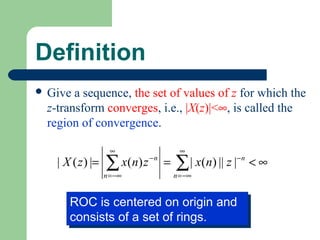
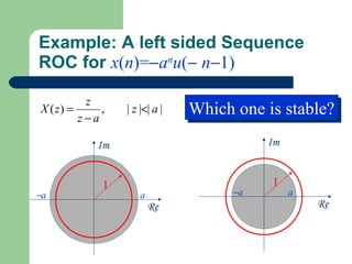
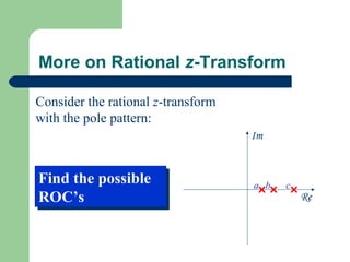
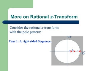
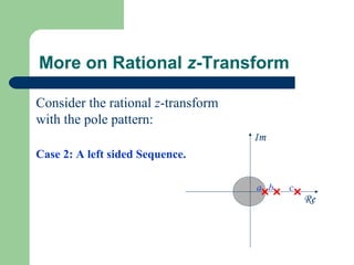
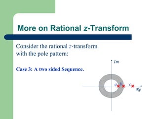
The z-transform provides a method to analyze discrete-time signals and systems using complex variable theory. It is defined as the summation of a sequence multiplied by z to the power of the time index from negative infinity to positive infinity. The region of convergence consists of values of z where this summation converges. It is determined by the locations of the zeros and poles of the z-transform function. Examples show how different sequences lead to different regions of convergence bounded by these zeros and poles.