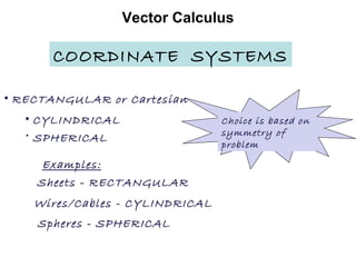
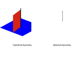
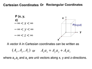
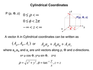
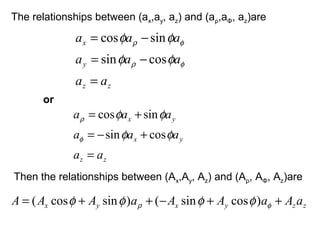
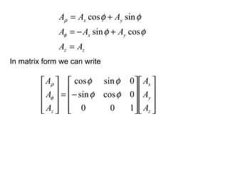
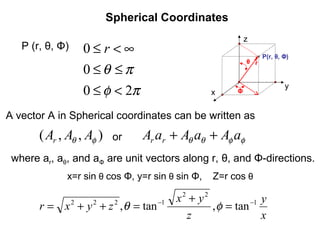
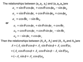
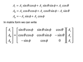
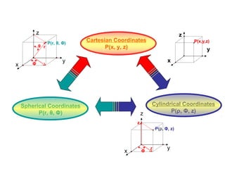
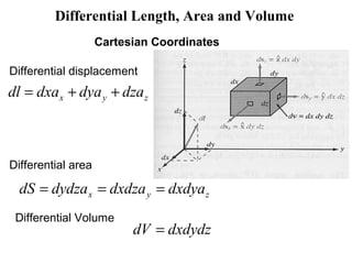
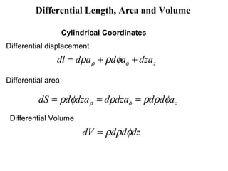
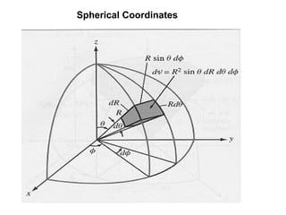
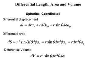
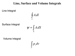
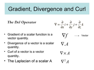
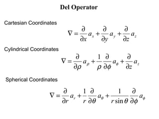
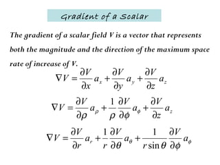
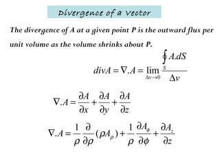
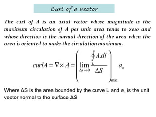
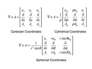
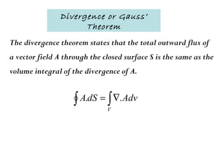
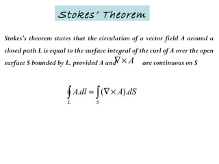
The document discusses vector calculus concepts including: 1) Coordinate systems used in vector calculus problems including rectangular, cylindrical, and spherical coordinates. 2) How to write vectors and their components in each coordinate system. 3) Relationships between vectors in different coordinate systems using transformation matrices. 4) Concepts of gradient, divergence, and curl and their definitions and representations in different coordinate systems. 5) Theorems relating integrals, including the divergence theorem and Stokes' theorem.

1. Vector Calculus

2. Vector Calculus
COORDINATE SYSTEMS
• RECTANGULAR or Cartesian
• CYLINDRICAL Choice is based on
• SPHERICAL symmetry of
problem
Examples:
Sheets - RECTANGULAR
Wires/Cables - CYLINDRICAL
Spheres - SPHERICAL

3. Cylindrical Symmetry Spherical Symmetry

4. Cartesian Coordinates Or Rectangular Coordinates
P (x, y, z
z)
−∞ < x < ∞ P(x,y,z)
−∞ < y < ∞
y
−∞ < z < ∞
x
A vector A in Cartesian coordinates can be written as
( Ax , Ay , Az ) or Ax a x + Ay a y + Az a z
where ax,ay and az are unit vectors along x, y and z-directions.

5. Cylindrical Coordinates
z
P (ρ, Φ, z)
0≤ρ <∞
z
P(ρ, Φ, z)
0 ≤ φ < 2π
−∞ < z < ∞ x Φ
ρ y
A vector A in Cylindrical coordinates can be written as
( Aρ , Aφ , Az ) or Aρ aρ + Aφ aφ + Az a z
where aρ,aΦ and az are unit vectors along ρ, Φ and z-directions.
x= ρ cos Φ, y=ρ sin Φ, z=z
y
ρ = x + y , φ = tan
2 2 −1
,z = z
x

6. The relationships between (ax,ay, az) and (aρ,aΦ, az)are
a x = cos φaρ − sin φaφ
a y = sin φaρ − cos φaφ
az = az
or
aρ = cos φa x + sin φa y
aφ = − sin φa x + cos φa y
az = az
Then the relationships between (Ax,Ay, Az) and (Aρ, AΦ, Az)are
A = ( Ax cos φ + Ay sin φ )aρ + (− Ax sin φ + Ay cos φ )aφ + Az a z

7. Aρ = Ax cos φ + Ay sin φ
Aφ = − Ax sin φ + Ay cos φ
Az = Az
In matrix form we can write
 Aρ   cos φ sin φ 0  Ax 
 A  = − sin φ cos φ 0  Ay 
 φ   
 Az   0
   0 1  Az 
 

8. Spherical Coordinates
z
P (r, θ, Φ) 0≤r <∞ P(r, θ, Φ)
θ r
0 ≤θ ≤π
0 ≤ φ < 2π x Φ
y
A vector A in Spherical coordinates can be written as
( Ar , Aθ , Aφ ) or Ar ar + Aθ aθ + Aφ aφ
where ar, aθ, and aΦ are unit vectors along r, θ, and Φ-directions.
x=r sin θ cos Φ, y=r sin θ sin Φ, Z=r cos θ
x2 + y2 −1 y
r = x 2 + y 2 + z 2 , θ = tan −1 , φ = tan
z x

9. The relationships between (ax,ay, az) and (ar,aθ,aΦ)are
a x = sin θ cos φar + cos θ cos φaθ − sin φaφ
a y = sin θ sin φar + cos θ sin φaθ + cos φaφ
a z = cos θar − sin θaθ
or
ar = sin θ cos φa x + sin θ sin φa y + cos θa z
aθ = cos θ cos φa x + cos θ sin φa y − sin θa z
aφ = − sin φa x + cos φa y
Then the relationships between (Ax,Ay, Az) and (Ar, Aθ,and AΦ)are
A = ( Ax sin θ cos φ + Ay sin θ sin φ + Az cos θ )ar
+ ( Ax cos θ cos φ + Ay cos θ sin φ − Az sin θ )aθ
+ (− Ax sin φ + Ay cos φ )aφ

10. Ar = Ax sin θ cos φ + Ay sin θ sin φ + Az cos θ
Aθ = Ax cos θ cos φ + Ay cos θ sin φ − Az sin θ
Aφ = − Ax sin φ + Ay cos φ
In matrix form we can write
 Ar   sin θ cos φ sin θ sin φ cos θ   Ax 
  
 Aθ  = cos θ cos φ cos θ sin φ − sin θ   Ay 
 
 Aφ   − sin φ cos φ 0   Az 
    

11. z z
P(r, θ, Φ)
Cartesian Coordinates P(x,y,z)
θ r P(x, y, z) y
y x
x Φ
Spherical Coordinates Cylindrical Coordinates
P(r, θ, Φ) z P(ρ, Φ, z)
z
P(ρ, Φ, z)
r y
x Φ

12. Differential Length, Area and Volume
Cartesian Coordinates
Differential displacement
dl = dxa x + dya y + dza z
Differential area
dS = dydza x = dxdza y = dxdya z
Differential Volume
dV = dxdydz

13. Cylindrical Coordinates
ρ ρ
ρ ρ
ρ
ρ ρρ
ρ
ρ ρ

14. Differential Length, Area and Volume
Cylindrical Coordinates
Differential displacement
dl = dρa ρ + ρdφaφ + dza z
Differential area
dS = ρdφdza ρ = dρdzaφ = ρdρdφa z
Differential Volume
dV = ρdρdφdz

15. Spherical Coordinates

16. Differential Length, Area and Volume
Spherical Coordinates
Differential displacement
dl = drar + rdθaθ + r sin θdφaφ
Differential area
dS = r sin θdθdφar = r sin θdrdφaθ = rdrdθaφ
2
Differential Volume
dV = r sin θdrdθdφ
2

17. Line, Surface and Volume Integrals
Line Integral
∫ A.dl
L
Surface Integral
ψ = ∫ A.dS
S
Volume Integral
∫ p dv
V
v

18. Gradient, Divergence and Curl
The Del Operator
• Gradient of a scalar function is a
vector quantity.
∇f Vector
• Divergence of a vector is a scalar
∇. A
quantity.
• Curl of a vector is a vector
∇× A
quantity.
• The Laplacian of a scalar A ∇ A
2

19. Del Operator
Cartesian Coordinates
∂ ∂ ∂
∇ = ax + a y + az
∂x ∂y ∂z
Cylindrical Coordinates
∂ 1 ∂ ∂
∇= aρ + aφ + a z
∂ρ ρ ∂φ ∂z
Spherical Coordinates
∂ 1 ∂ 1 ∂
∇ = ar + aθ + aφ
∂r r ∂θ r sin θ ∂φ

20. Gradient of a Scalar
The gradient of a scalar field V is a vector that represents
both the magnitude and the direction of the maximum space
rate of increase of V.
∂V ∂V ∂V
∇V = ax + ay + az
∂x ∂y ∂z
∂V 1 ∂V ∂V
∇V = aρ + aφ + az
∂ρ ρ ∂φ ∂z
∂V 1 ∂V 1 ∂V
∇V = ar + aθ + aφ
∂r r ∂θ r sin θ ∂φ

21. Divergence of a Vector
The divergence of A at a given point P is the outward flux per
unit volume as the volume shrinks about P.
∫ A.dS
divA = ∇. A = lim S
∆v →0 ∆v
∂A ∂A ∂A
∇. A = + +
∂x ∂y ∂z
1 ∂ 1 ∂Aφ ∂Az
∇. A = ( ρAρ ) + +
ρ ∂ρ ρ ∂φ ∂z

22. Curl of a Vector
The curl of A is an axial vector whose magnitude is the
maximum circulation of A per unit area tends to zero and
whose direction is the normal direction of the area when the
area is oriented to make the circulation maximum.
 A.dl 
 ∫ 
curlA = ∇ × A =  lim L  an
 ∆s →0 ∆S 
 
  max
Where ΔS is the area bounded by the curve L and an is the unit
vector normal to the surface ΔS

23.  ax ay az   aρ ρaφ az 
∂ ∂ ∂ 1∂ ∂ ∂
∇× A =   ∇× A =  
 ∂x ∂y ∂z  ρ  ∂ρ ∂φ ∂z 
 Ax
 Ay Az 
  Aρ
 ρAφ Az 

Cartesian Coordinates Cylindrical Coordinates
 ar raθ r sin θaφ 
1 ∂ ∂ ∂ 
∇× A = 2  
r sin θ  ∂r ∂θ ∂φ 
 Ar
 rAθ r sin θAφ 

Spherical Coordinates

24. Divergence or Gauss’
Theorem
The divergence theorem states that the total outward flux of
a vector field A through the closed surface S is the same as the
volume integral of the divergence of A.
∫ A.dS = ∫ ∇. Adv
V

25. Stokes’ Theorem
Stokes’s theorem states that the circulation of a vector field A around a
closed path L is equal to the surface integral of the curl of A over the open
surface S bounded by L, provided A and × A
∇ are continuous on S
∫ A.dl = ∫ (∇ × A).dS
L S