The document derives Bresenham's line algorithm for drawing lines on a discrete grid. It starts with the line equation and defines variables for the slope and intercept. It then calculates the distance d1 and d2 from the line to two possible pixel locations and expresses their difference in terms of the slope and intercept. By multiplying this difference by the change in x, it removes the floating point slope value, resulting in an integer comparison expression. This is defined recursively to draw each subsequent pixel, using pre-computed constants. The initial p0 value is also derived from the line endpoint coordinates.

1. Appendix: Derivation of Bresenham’s line algorithm
© E Claridge, School of Computer Science, The University of Birmingham
DERIVATION OF THE BRESENHAM’S LINE ALGORITHM
Assumptions:
● input: line endpoints at (X1,Y1) and (X2, Y2)
● X1 < X2
● line slope ≤ 45o
, i.e. 0 < m ≤ 1
● x coordinate is incremented in steps of 1, y coordinate is computed
● generic line equation: y = mx + b
x x +1i i
y i
y +1i
y = mx + b
y
d1
d2
Derivation
Assume that we already have a location of pixel ( xi, yi) and have plotted it. The question is,
what is the location of the next pixel.
Geometric location of the line at x-coordinate xi+1 = xi + 1 is:
y = m(xi + 1 ) + b (1)
where:
m = ∆y / ∆x (slope) (2)
b – intercept
∆x = X2 – X1 (from the assumption above that X1 < X2 ) (3)
∆y = Y2 – Y1
Define:
d1 = y – yi = m(xi + 1 ) + b - yi
d2 = ( yi + 1 ) - y = yi + 1 - m(xi + 1 ) - b
Calculate:
d1 – d2 = m(xi + 1 ) + b - yi - yi – 1 + m(xi + 1 ) + b
= 2m(xi + 1 ) – 2yi + 2b – 1 (4)
if d1 – d2 < 0 then yi+1 ← yi (5)
if d1 – d2 > 0 then yi+1 ← yi + 1 (6)
We want integer calculations in the loop, but m is not an integer. Looking at definition of m
(m = ∆y / ∆x) we see that if we multiply m by ∆x, we shall remove the denominator and
hence the floating point number.

2. Appendix: Derivation of Bresenham’s line algorithm
© E Claridge, School of Computer Science, The University of Birmingham
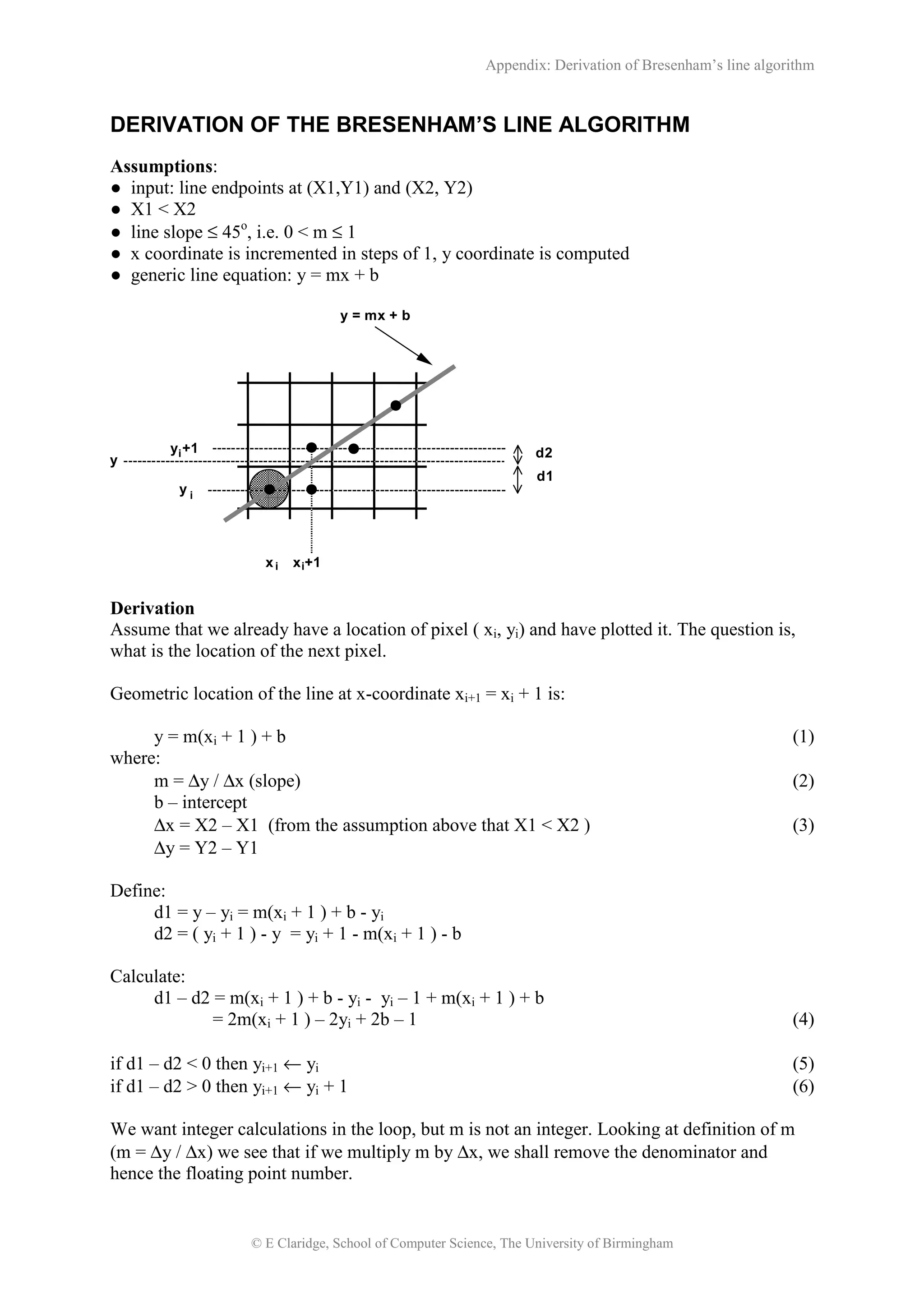
For this purpose, let us multiply the difference ( d1 - d2 ) by ∆x and call it pi:
pi = ∆x( d1 – d2)
The sign of pi is the same as the sign of d1 – d2, because of the assumption (3).
Expand pi:
pi = ∆x( d1 – d2)
= ∆x[ 2m(xi + 1 ) – 2yi + 2b – 1 ] from (4)
= ∆x[ 2 ⋅ (∆y / ∆x ) ⋅ (xi + 1 ) – 2yi + 2b – 1 ] from (2)
= 2⋅∆y⋅ (xi + 1 ) – 2⋅∆x⋅yi + 2⋅∆x⋅b – ∆x result of multiplication by ∆x
= 2⋅∆y⋅xi + 2⋅∆y – 2⋅∆x⋅yi + 2⋅∆x⋅b – ∆x
= 2⋅∆y⋅xi– 2⋅∆x⋅yi + 2⋅∆y + 2⋅∆x⋅b – ∆x (7)
Note that the underlined part is constant (it does not change during iteration), we call it c, i.e.
c = 2⋅∆y + 2⋅∆x⋅b – ∆x
Hence we can write an expression for pi as:
pi = 2⋅∆y⋅xi– 2⋅∆x⋅yi + c (8)
Because the sign of pi is the same as the sign of d1 – d2, we could use it inside the loop to
decide whether to select pixel at (xi + 1, yi ) or at (xi + 1, yi +1). Note that the loop will only
include integer arithmetic. There are now 6 multiplications, two additions and one selection in
each turn of the loop.
However, we can do better than this, by defining pi recursively.
pi+1 = 2⋅∆y⋅xi+1– 2⋅∆x⋅yi+1 + c from (8)
pi+1 – pi = 2⋅∆y⋅xi+1– 2⋅∆x⋅yi+1 + c
- (2⋅∆y⋅xi – 2⋅∆x⋅yi + c )
= 2∆y ⋅ (xi+1 – xi) – 2∆x ⋅ (yi+1 – yi) xi+1 – xi = 1 always
pi+1 – pi = 2∆y – 2∆x ⋅ (yi+1 – yi)
Recursive definition for pi:
pi+1 = pi + 2∆y – 2∆x ⋅ (yi+1 – yi)
If you now recall the way we construct the line pixel by pixel, you will realise that the
underlined expression: yi+1 – yi can be either 0 ( when the next pixel is plotted at the same y-
coordinate, i.e. d1 – d2 < 0 from (5)); or 1 ( when the next pixel is plotted at the next y-
coordinate, i.e. d1 – d2 > 0 from (6)). Therefore the final recursive definition for pi will be
based on choice, as follows (remember that the sign of pi is the same as the sign of d1 – d2):

3. Appendix: Derivation of Bresenham’s line algorithm
© E Claridge, School of Computer Science, The University of Birmingham
if pi < 0, pi+1 = pi + 2∆y because 2∆x ⋅ (yi+1 – yi) = 0
if pi > 0, pi+1 = pi + 2∆y – 2∆x because (yi+1 – yi) = 1
At this stage the basic algorithm is defined. We only need to calculate the initial value for
parameter po.
pi = 2⋅∆y⋅xi– 2⋅∆x⋅yi + 2⋅∆y + 2⋅∆x⋅b – ∆x from (7)
p0 = 2⋅∆y⋅x0– 2⋅∆x⋅y0 + 2⋅∆y + 2∆x⋅b – ∆x (9)
For the initial point on the line:
y0 = mx0 + b
therefore
b = y0 – (∆y/∆x) ⋅ x0
Substituting the above for b in (9)we get:
p0 = 2⋅∆y⋅x0– 2⋅∆x⋅y0 + 2⋅∆y + 2∆x⋅ [ y0 – (∆y/∆x) ⋅ x0 ] – ∆x
= 2⋅∆y⋅x0 – 2⋅∆x⋅y0 + 2⋅∆y + 2∆x⋅y0 – 2∆x⋅ (∆y/∆x) ⋅ x0 – ∆x simplify
= 2⋅∆y⋅x0 – 2⋅∆x⋅y0 + 2⋅∆y + 2∆x⋅y0 – 2∆y⋅x0 – ∆x regroup
= 2⋅∆y⋅x0 – 2∆y⋅x0 – 2⋅∆x⋅y0 + 2∆x⋅y0 + 2⋅∆y – ∆x simplify
= 2⋅∆y – ∆x
We can now write an outline of the complete algorithm.
Algorithm
1. Input line endpoints, (X1,Y1) and (X2, Y2)
2. Calculate constants:
∆x = X2 – X1
∆y = Y2 – Y1
2∆y
2∆y – ∆x
3. Assign value to the starting parameters:
k = 0
p0 = 2∆y – ∆x
4. Plot the pixel at ((X1,Y1)
5. For each integer x-coordinate, xk, along the line
if pk < 0 plot pixel at ( xk + 1, yk )
pk+1 = pk + 2∆y (note that 2∆y is a pre-computed constant)
else plot pixel at ( xk + 1, yk + 1 )
pk+1 = pk + 2∆y – 2∆x
(note that 2∆y – 2∆x is a pre-computed constant)
increment k
while xk < X2