Downloaded 30 times


![38
of
60
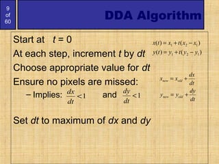
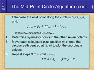
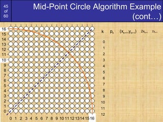
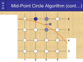
Mid-Point Circle Algorithm (cont…)
To ensure things are as efficient as possible
we can do all of our calculations
incrementally
First consider:
or:
where yk+1 is either yk or yk-1 depending on
the sign of p
( )
( ) 2
2
1
2
111
2
1]1)1[(
2
1,1
ryx
yxfp
kk
kkcirck
−−+++=
−+=
+
+++
1)()()1(2 1
22
11 +−−−+++= +++ kkkkkkk yyyyxpp](https://image.slidesharecdn.com/bresenhamcirclesandpolygons-150603132413-lva1-app6892/85/Bresenham-circles-and-polygons-derication-37-320.jpg)
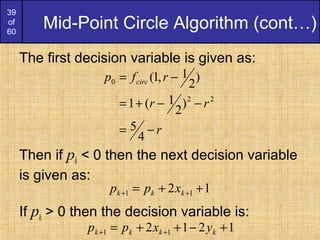


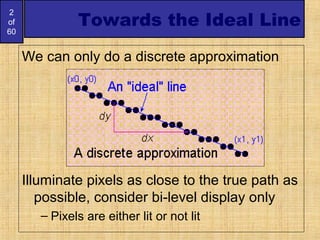
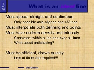
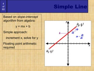
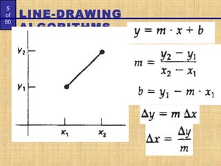
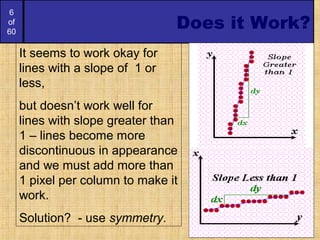
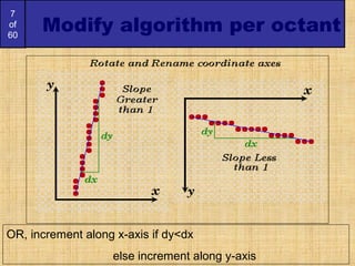
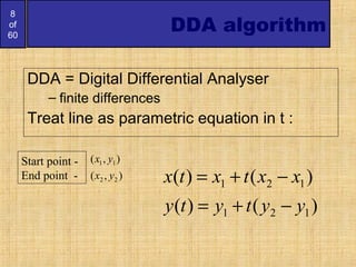
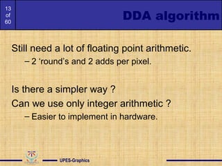
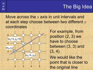
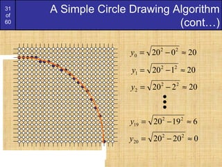
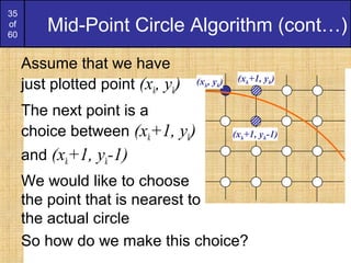
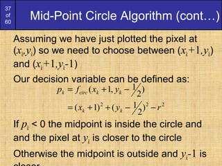
The document discusses algorithms for drawing lines and circles on a discrete pixel display. It begins by describing what characteristics an "ideal line" would have on such a display. It then introduces several algorithms for drawing lines, including the simple line algorithm, digital differential analyzer (DDA) algorithm, and Bresenham's line algorithm. The Bresenham algorithm is described in detail, as it uses only integer calculations. Next, a simple potential circle drawing algorithm is presented and its shortcomings discussed. Finally, the more accurate and efficient mid-point circle algorithm is described. This algorithm exploits the eight-way symmetry of circles and uses incremental calculations to determine the next pixel point.


![Chapter 3 - Part 1 [Autosaved].pptx](https://cdn.slidesharecdn.com/ss_thumbnails/chapter3-part1autosaved-230109040832-9344385c-thumbnail.jpg?width=640&height=640&fit=bounds)