HFS 3283 independent t test

HFS3283
INDEPENDENT T-TEST
DR. SHARIFAH WAJIHAH WAFA BTE SST WAFA
School of Nutrition and Dietetics
Faculty of Health Sciences
sharifahwajihah@unisza.edu.my
KNOWLEDGE FOR THE BENEFIT OF HUMANITY

SCHOOL OF NUTRITION AND DIETETICS . FACULTY OF HEALTH SCIENCES
Topic Learning Outcomes
At the end of this lecture, the student should be
able to:
1
• Understand structure of research study appropriate
for independent-measures t hypothesis test
2
• Test between two populations or two treatments
using independent-measures t statistics
3
• Understand how to evaluate the assumptions
underlying this test

Independent-measures Design
Introduction
• Most research studies compare two (or more)
sets of data
– Data from two completely different, independent
participant groups (an independent-measures or
between-subjects design)
– Data from the same or related participant group(s)
(a within-subjects or repeated-measures design)

Independent-Measures Design
Introduction (continued)
• Computational procedures are considerably
different for the two designs
• Each design has different strengths and
weaknesses
• Consequently, only between-subjects designs
are considered in this lecture; repeated-
measures designs will be reserved for
discussion in Next Lecture

When to use the independent
samples t-test
• It is used to compare differences between separate
groups.
• This test can be used to explore differences in
naturally occurring groups.
• For example, we may be interested in differences of
IQ between males and females.

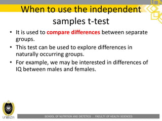
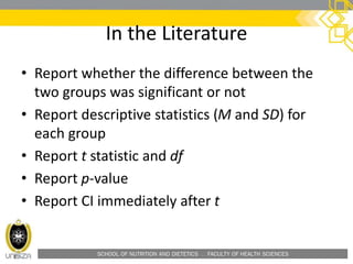
When to use the independent
samples t-test (cont.)
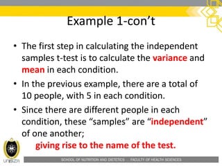
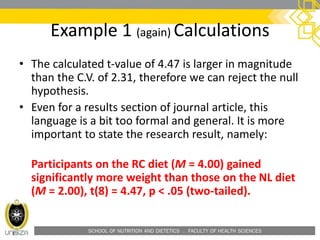
• Any differences between groups can be
explored with the independent t-test, as long
as the tested members of each group are
reasonably representative of the population.
[1]
[1] There are some technical
requirements as well. Principally,
each variable must come from a
normal (or nearly normal) distribution.

Independent-Measures Design t
Statistic
• Null hypothesis for independent-measures
test
• Alternative hypothesis for the independent-
measures test
0: 210  H
0: 211  H

Example 1
• Suppose we put people on 2 diets:
the nasi lemak diet and the roti canai diet.
• Participants are randomly assigned to either 1-
week of breakfast eating exclusively nasi (NL)
lemak or 1-week of exclusively roti canai (RC).

Example 1-con’t
• At the end of the week, we measure
weight gain by each participant.
• Which diet causes more weight gain?
• In other words, the null hypothesis is:
Ho: wt. gain NL diet =wt. gain RC diet.

Example 1-con’t
• Why?
• The null hypothesis is the opposite of what we
hope to find.
• In this case, our research hypothesis is that
there ARE differences between the 2 diets.
• Therefore, our null hypothesis is that there are
NO differences between these 2 diets.

Example 1-con’t
Column 3 Column 4
X1 : NL X2 : RC
1 3 1 1
2 4 0 0
2 4 0 0
2 4 0 0
3 5 1 1
2 4
0.4 0.4
2
11 )(  2
22 )( 
1
2




n
sx
2
2
)(

Example 1-con’t
• The first step in calculating the independent
samples t-test is to calculate the variance and
mean in each condition.
• In the previous example, there are a total of
10 people, with 5 in each condition.
• Since there are different people in each
condition, these “samples” are “independent”
of one another;
giving rise to the name of the test.

Example 1-con’t
• The variances and means are calculated
separately for each condition
(NL and RC).
• A streamlined calculation of the variance for
each condition was illustrated previously. (See
Slide 11.)
• In short, we take each observed weight gain
for the NL condition, subtract it from the
mean gain of the NL dieters ( 2) and
square the result (see column 3).
1

Example 1-con’t
• Next, add up column 3 and divide by the
number of participants in that condition (n1 =
5) to get the sample variance,
• The same calculations are repeated for the
“RC” condition.
4.02
xs

Formula
The formula for
the independent samples t-test is:
, df = (n1-1) + (n2-1)
11 2
2
1
2
21
21





n
S
n
S
t
xx

Example 1 (cont.)
• Where
= Mean of first sample
= Mean of second sample
n1 = Sample size (i.e., number of observations) of
first sample
n2 = Sample size (i.e., number of observations) of
second sample
= sample variance of first sample
= sample variance of second sample
sp = Pooled standard deviation
2
1xs
2
2xs
1
2

Example 1 (cont.)
• From the calculations previously, we have
everything that is needed to find the “t.”
47.4
4
4.
4
4.
42



t , df = (5-1) + (5-1) = 8
• After calculating the “t” value, we need to
know if it is large enough to reject the null
hypothesis.

• The “t” is calculated under the assumption,
called the null hypothesis,
“that there are no differences between
the NL and RC diet”.
• If this were true, when we repeatedly sample
10 people from the population and put them
in our 2 diets, most often we would calculate
a “t” of “0.”
Some theory

• Look again at the formula for the “t”.
• Most often the numerator (X1-X2) will be “0,”
because the mean of the two conditions
should be the same under the null hypothesis.
• That is, weight gain is the same under both
the NL and RC diet.
Some theory - Why?

• Sometimes the weight gain might be a bit
higher under the NL diet, leading to a positive
“t” value.
• In other samples of 10 people, weight gain
might be a little higher under the RC diet,
leading to a negative “t” value.
• The important point, however, is that under
the null hypothesis we should expect that
most “t” values that we compute are close to
“0.”
Some theory - Why (cont.)

• Our computed t-value is not “0,” but it is in fact
negative (t(8) = -4.47).
• Although the t-value is negative, this should not
bother us.
• Remember that the t-value is only - 4.47 because we
named the NL diet X1 and the RC diet X2.
–This is, of course, completely arbitrary.
• If we had reversed our order of calculation, with the
NL diet as X2 and the RC diet as X1, then our
calculated t-value would be positive 4.47.
Some theory - Why (cont.)

• The calculated t-value is 4.47 (notice, I’ve
eliminated the unnecessary “-“ sign), and the
degrees of freedom are 8.
• In the research question we did not specify
which diet should cause more weight gain,
therefore this t-test is a so-called “2-tailed t.”
Example 1 (again) Calculations

Degrees of freedom
• Degrees of freedom (df) for t statistic is
df for first sample + df for second sample
)1()1( 2121  nndfdfdf
Note: this term is the same as the denominator of the pooled
variance

• In the last step, we need to find the critical
value for a 2-tailed “t” with 8 degrees of
freedom.
• This is available from tables that are in the
back of any Statistics textbook.
• Look in the back for “Critical Values of the t-
distribution,” or something similar.
• The value you should find is:
C.V. t(8), 2-tailed = 2.31.

• The calculated t-value of 4.47 is larger in magnitude
than the C.V. of 2.31, therefore we can reject the null
hypothesis.
• Even for a results section of journal article, this
language is a bit too formal and general. It is more
important to state the research result, namely:
Participants on the RC diet (M = 4.00) gained
significantly more weight than those on the NL diet
(M = 2.00), t(8) = 4.47, p < .05 (two-tailed).

Repeat from previous slide:
significantly more weight than those on the
NL diet (M = 2.00), t(8) = 4.47, p < .05 (two-
tailed).
• Making this conclusion requires inspection of
the mean scores for each condition (NL and
RC).
Example 1 (concluding comment)

Example 1 Using SPSS
• First, the variables must be setup in the SPSS data
editor.
• We need to include both the independent and
dependent variables.
• Although it is not strictly necessary, it is good
practice to give each person a unique code
(e.g., personid):

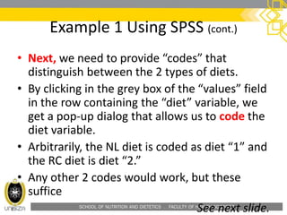
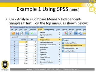
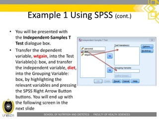
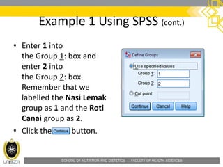
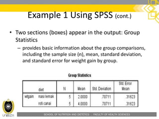
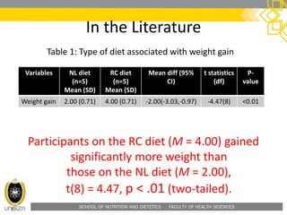
Example 1 Using SPSS (cont.)
• In the previous example:
– Dependent Variable
= wtgain (or weight gain)
– Independent Variable = diet
• Why?
• The independent variable (diet) causes
changes in the dependent variable (weight
gain).

• Next, we need to provide “codes” that
distinguish between the 2 types of diets.
• By clicking in the grey box of the “values” field
in the row containing the “diet” variable, we
get a pop-up dialog that allows us to code the
diet variable.
• Arbitrarily, the NL diet is coded as diet “1” and
the RC diet is diet “2.”
• Any other 2 codes would work, but these
suffice
See next slide.

.

• Moving to the data view
tab of the SPSS editor,
the data is entered.
• Each participant is
entered on a separate
line; a code is entered
for the diet they were
on (1 = NL, 2 = RC); and
the weight gain of each
is entered, as follows 

• Click Analyze > Compare Means > Independent-
Samples T Test... on the top menu, as shown below:

• You will be presented with
the Independent-Samples T
Test dialogue box.
• Transfer the dependent
variable, wtgain, into the Test
Variable(s): box, and transfer
the independent variable, diet,
into the Grouping Variable:
box, by highlighting the
relevant variables and pressing
the SPSS Right Arrow Button
buttons. You will end up with
the following screen in the
next slide

You then need to define the groups (diet). Click on
the button. You will be presented with the Define
Groups dialogue box, as shown above:

• Enter 1 into
the Group 1: box and
enter 2 into
the Group 2: box.
Remember that we
labelled the Nasi Lemak
group as 1 and the Roti
Canai group as 2.
• Click the button.

• Two sections (boxes) appear in the output: Group
Statistics
– provides basic information about the group comparisons,
including the sample size (n), mean, standard deviation,
and standard error for weight gain by group.

• SPSS gives the means for each of the conditions
(NL Mean = 2 and RC Mean = 4).
• In addition, SPSS provides a t-value of -4.47 with
8 degrees of freedom.
• These are the same figures that were computed
“by hand” previously.
• However, SPSS does not provide a critical value.
• Instead, an exact probability is provided (p =
.002).

• The second section, Independent Samples Test, displays the
results most relevant to the Independent Samples t Test.
There are two parts that provide different pieces of
information: (A) Levene’s Test for Equality of Variances and (B)
t-test for Equality of Means.

Levene's Test for Equality of of Variances: This section has the test results for
Levene's Test. From left to right:
• F is the test statistic of Levene's test
• Sig. is the p-value corresponding to this test statistic.
The p-value of Levene's test is printed as “1.000“, so we ACCEPT the null of Levene's
test and conclude that the variance in weight gain of NL diet is identical to the RC
diet .This tells us that we should look at the "Equal variances assumed" row for the
t-test results. (If this test result had been significant -- that is, if we had
observed p < α -- then we would have used the "Equal variances not assumed"
output.)

t-test for Equality of Means provides the results for the actual Independent
Samples t Test. From left to right:
• t is the computed test statistic
• df is the degrees of freedom
• Sig (2-tailed) is the p-value corresponding to the given test statistic and degrees
of freedom
• Mean Difference is the difference between the sample means; it also
corresponds to the numerator of the test statistic
• Std. Error Difference is the standard error; it also corresponds to the
denominator of the test statistic

• The mean difference is calculated by subtracting the mean of the second group
from the mean of the first group. In this example, the mean weight gain for RC
diet was subtracted from the mean weight gain for NL diet (2.00- 4.00 = -2.00).
The sign of the mean difference corresponds to the sign of the t value.
• The negative t value in this example indicates that the mean weight gain for the
first group, NL diet, is significantly lower than the mean for the second group, RC
diet.
• The associated p value is printed as ".002".

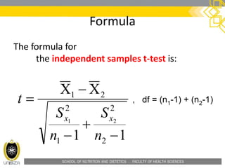
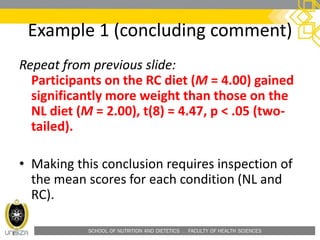
• Confidence Interval of the Difference: This part of the t-test output
complements the significance test results. Typically, if the CI for the mean
difference contains 0, the results are not significant at the chosen significance
level. In this example, the CI is [-3.03128, -0.96872], which does not contain
zero; this agrees with the small p-value of the significance test.

In the Literature
• Report whether the difference between the
two groups was significant or not
• Report descriptive statistics (M and SD) for
each group
• Report t statistic and df
• Report p-value
• Report CI immediately after t

In the Literature
significantly more weight than
those on the NL diet (M = 2.00),
t(8) = 4.47, p < .01 (two-tailed).
Variables NL diet
(n=5)
Mean (SD)
RC diet
(n=5)
Mean (SD)
Mean diff (95%
CI)
t statistics
(df)
P-
value
Weight gain 2.00 (0.71) 4.00 (0.71) -2.00(-3.03,-0.97) -4.47(8) <0.01
Table 1: Type of diet associated with weight gain

Repeat from previous slide:
significantly more weight than those on the NL diet
(M = 2.00), t(8) = 4.47, p < .01 (two-tailed).
• In APA style we normally only display significance to
2 significant digits.
• Therefore, the probability is displayed as “p<.01,”
which is the smallest probability within this range of
accuracy.

Sample size??
• In each group, sample size is BIG (>30)
• In case, the sample size is less than 30 in one group,
so that we need to check for normality assumption.
• How to check?

Normality assumption

recap
• FOUR assumptions
1. Random sample
2. Observations are independent
3. In each group, data are normally distributed or
sample size is big (>30)
4. Population variances are not different between
2 groups Levene’s test

Any
Questio
ns?
Conce
pts?
Equations?

HFS 3283 independent t test

Recommended

Recommended

More Related Content

What's hot

What's hot (20)

Viewers also liked

Viewers also liked (20)

Similar to HFS 3283 independent t test

Similar to HFS 3283 independent t test (20)

More from wajihahwafa

More from wajihahwafa (20)

Recently uploaded

Recently uploaded (20)

HFS 3283 independent t test