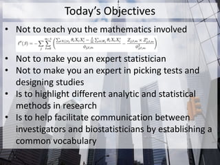
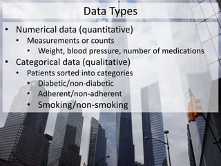
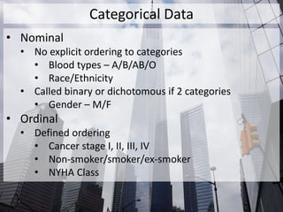
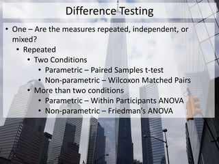
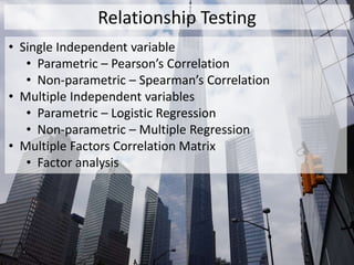
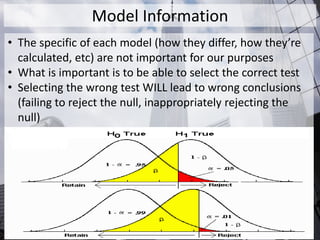
The document outlines the fundamentals of statistical analysis, emphasizing the importance of understanding different data types and methods to facilitate communication between researchers and biostatisticians. It covers key concepts such as data types (numerical and categorical), statistical inference, hypothesis testing, and the selection of appropriate tests based on the nature of the data. Additionally, it highlights the distinction between parametric and nonparametric methods, stressing the need for careful test selection to avoid incorrect conclusions.

1. Analysis 101
Brian Wells

2. Today’s Objectives
• Not to teach you the mathematics involved
• Not to make you an expert statistician
• Not to make you an expert in picking tests and
designing studies
• Is to highlight different analytic and statistical
methods in research
• Is to help facilitate communication between
investigators and biostatisticians by establishing a
common vocabulary

3. Data Types
• Numerical data (quantitative)
• Measurements or counts
• Weight, blood pressure, number of medications
• Categorical data (qualitative)
• Patients sorted into categories
• Diabetic/non-diabetic
• Adherent/non-adherent
• Smoking/non-smoking

4. Categorical Data
• Nominal
• No explicit ordering to categories
• Blood types – A/B/AB/O
• Race/Ethnicity
• Called binary or dichotomous if 2 categories
• Gender – M/F
• Ordinal
• Defined ordering
• Cancer stage I, II, III, IV
• Non-smoker/smoker/ex-smoker
• NYHA Class

5. Numerical Data
• Can be further subdivided into discrete and
continuous
• Discrete variables
• Have a limited number of possible values (finite or
countably infinite)
• Gaps between possible values (whole integers)
• Ex: Number of CHF episodes, number of medications
• Continuous variables
• No gaps between possible values
• Ex: Duration of seizure, body mass index, height

6. Determining Data Types
• Ordinal (Categorical) v. Discrete (Numerical)
• Ordinal
• Cancer Stage I, II, III, IV
• Cancer Stage II is not 2*Stage I
• Discrete
• Number of children: 0, 1, 2…
• 4 children = 2 times 2 children

7. So Why Spend Time On This?
• The data types help determine which analysis to
use
• It helps determine how best to summarize the
display data
• Categorical – percent's, fractions, numbers in
categories
• Numerical – mean, median, mode, standard
deviation, variance, quartile ranges

8. Data Summaries
• Be careful of overreliance on numbers – Keep the
big picture in mind (more on this next time)
• Both means = 2, SD = 1.9, n = 1000

9. Statistical Inference
• Estimation of quantity of interest
• Estimate itself
• Quantify how good an estimate it is
• Ex: If you took more and more samples, how much
would the estimate vary?
• Hypothesis testing

10. Statistical Inference Example
• Proportion of people in a population who have diabetes.
N = 800
• Sample 1: 200/800 = 0.25
• We conclude that the estimated % of people with
diabetes is 25%
• But how variable is our estimate?
• We need to know the sampling distribution!
• Option 1: Take lots and lots of samples
• Sample 2: 215/800 = 26.8%
• Sample 3: 194/800 = 24.25%
• Not practical!

11. Statistical Inference Example
• Statistical theory
• Sample distributions for means and proportions are
normally “bell-shaped”
• From a single sample, we calculate the standard error
(variability) of our estimated mean or proportion
• Standard error measures the variability of the sample
statistic. Small SE means more precise estimate.
• SE ≠ Standard Deviation
• SD = variability of the sample data
• SE = variability of the statistic

12. Distributions
• Sample means follow a t-distributions on if
• Underlying data is approximately normal OR
• N is large
• A sample mean from a sample of size n will have a t
distributions with n-1 degrees of freedom (tn-1)

13. Confidence Intervals
• Assume we use our t15 distribution with n = 16, mean SBP
= 123.4 mm Hg, and SD = 14.0 mm Hg
• SE of mean = SD / √n = 3.5
• 95% CI for sample mean is then
• Mean + 2.131 (for t15 distribution) * SE
• = 123.4 ± 2.131 * SE
• = (115.9, 130.8) mm Hg
• And as N gets larger, t statistic gets smaller (t99 = 1.984),
which with the same numbers as above but with N = 100,
CI narrows to (120.6, 126.2)
• Note: It’s never incorrect to use a t-distribution as long as
the underlying population is normal or N is large

14. Hypothesis Testing
• Confidence intervals told us the best estimate and the
variability of the best estimate
• Hypothesis testing tells us if there really is a difference
between an observed value and another value
• From our earlier example: N = 800, we estimated that
25% of people had diabetes
• Let’s say a study 10 years prior estimated that 12% of
people had diabetes
• Has the percent of people with diabetes really changed?

15. Hypothesis Testing
• Support the true percent of people with diabetes is 12%
• Called the null hypothesis or H0
• How likely is it that we would observe a result as or more
extreme than 25% given the true percent is 12%?
• This is the p-value, computed using normal distributions for
sample proportions and t-distribution for sample means
• If the probability is small, consult the supposition may not be
right
• Reject the null hypothesis in favor of the alternate
hypothesis Ha
• If the probability is not small, conclude that there is
insufficient evidence to reject the null hypothesis
• This is NOT the same as accepting the null or showing the
null hypothesis is true

16. Hypothesis Testing
• H0: True proportion is 12%
• Ha: True proportion is not 12%
• If P < 0.05, we would conclude it is not likely to observe
our data is the true proportion was 12%
• We conclude that this is sufficient evidence that the
proportion with diabetes is not 12%
• Test can be one-sided or two-sided
• One-sided ONLY ok if previous research suggests that the
proportion is larger

17. Misinterpreting the p-value
• A p-value of 0.32 (or > 0.05) DOES NOT mean:
• We accept the null
• There is a 32% chance the null is true
• It only lets us reject the null in favor of the alternative or
fail to reject the null
• If you fail to reject, it DOES NOT mean the alternative isn’t
true. It may mean your N is too small or the study is
underpowered.

18. Decision-Making

19. Other Statistics
• Some statistics are distribution-free
• Recall that t-tests/distributions depend on normality or
large N’s
• What is we don’t have one or both of these, ex: skewed
data, N is small
• We can use nonparametric methods that look at ranks,
not means
• The median is a nonparametric estimate

20. Nonparametric Methods
• Don’t require a particular distribution
• Well-suited to hypothesis testing
• Not as useful for point estimates or Cis
• Especially useful is data is ranks or scores – Apgar scores,
Vision (20/20, 20/40)
• Do inferences on medial values
• Hypothesis Test is Sign Test
• Assumes hypothesized value of median is correct,
except to observe about half the sample above and
half below
• Computes probability for proportion above median

21. Parametric v. Nonparametric
• Nonparametric are always ok to use
• Nonparametric are more conservative than parametric
• In fact, 95% CI for medians are sometimes twice as
wide as those for the mean
• If your N is fairly large, or if you know your data is normal,
parametric is always best

22. How To Select A Test
• Start by asking, “Am I testing for a difference or a
relationship in my data?”

23. Difference Testing
• Am I testing one sample or more than one sample?
• One sample – Is my data parametric?
• Yes – One sample t-test
• No – Wilcoxon Signed Rank Test

24. Difference Testing
• More than one sample – Is my data nominal, or
ordinal/interval/ratio?
• Nominal – Chi-Squared test
• Ordinal/interval/ratio – How many dependent
variables are there?
• Two or more – Multivariate Analysis of Variance
(MANOVA)

25. Difference Testing
• One – Are the measures repeated, independent, or
mixed?
• Mixed – Mixed Model ANOVA
• Independent
• How many conditions are there?
• Two conditions
• Parametric data – Independent samples t-test
• Non-parametric data – Mann-Whitney U test
• More than two
• Parametric – Between Participants (One-Way)
ANOVA
• Non-parametric – Kruskal-Wallis
• Repeated

26. Difference Testing
• One – Are the measures repeated, independent, or
mixed?
• Repeated
• Two Conditions
• Parametric – Paired Samples t-test
• Non-parametric – Wilcoxon Matched Pairs
• More than two conditions
• Parametric – Within Participants ANOVA
• Non-parametric – Friedman’s ANOVA

27. Relationship Testing
• Single Independent variable
• Parametric – Pearson’s Correlation
• Non-parametric – Spearman’s Correlation
• Multiple Independent variables
• Parametric – Logistic Regression
• Non-parametric – Multiple Regression
• Multiple Factors Correlation Matrix
• Factor analysis

28. Model Information
• The specific of each model (how they differ, how they’re
calculated, etc) are not important for our purposes
• What is important is to be able to select the correct test
• Selecting the wrong test WILL lead to wrong conclusions
(failing to reject the null, inappropriately rejecting the
null)

29. Going Further
• There are many, many more tests we did not cover
• Durbin-Watson
• Kolmogorov-Smirnov
• Anderson-Darling
• Cox Proportional Hazards
• Kaplan-Meier Survival Analysis
• And so on…
• However, the tests presented will cover the majority of
basic studies done