Downloaded 207 times
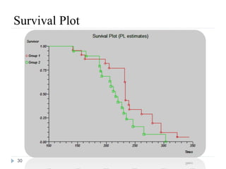
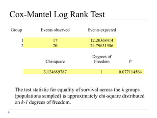
![India: 2010
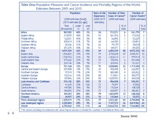
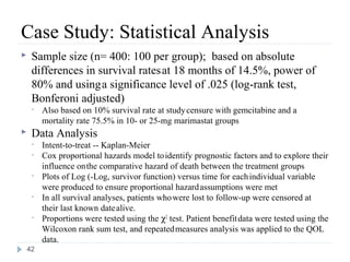
7137 of 122 429 study deaths were due to cancer, corresponding to 556 400 national
cancer deaths in India in 2010.
395 400 (71%) cancer deaths occurred in people aged 30—69 years (200 100 men
and 195 300 women).
At 30—69 years, the three most common fatal cancers were oral (including lip and
pharynx, 45 800 [22·9%]), stomach (25 200 [12·6%]), and lung (including trachea
and larynx, 22 900 [11·4%]) in men, and cervical (33 400 [17·1%]), stomach
(27 500 [14·1%]), and breast (19 900 [10·2%]) in women.
Tobacco-related cancers represented 42·0% (84 000) of male and 18·3% (35 700) of
female cancer deaths and there were twice as many deaths from oral cancers as lung
cancers.
Age-standardized cancer mortality rates per 100 000 were similar in rural (men 95·6
[99% CI 89·6—101·7] and women 96·6 [90·7—102·6]) and urban areas (men 102·4
[92·7—112·1] and women 91·2 [81·9—100·5]), but varied greatly between the
states.
Cervical cancer was far less common in Muslim than in Hindu women (study deaths
24, age-standardized mortality ratio 0·68 [0·64—0·71] vs 340, 1·06 [1·05—1·08]).
8](https://image.slidesharecdn.com/survcoxsardarpatelunivpart1final-130130010854-phpapp02/85/Part-1-Survival-Analysis-7-320.jpg)
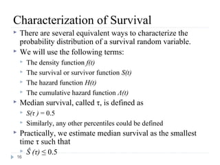
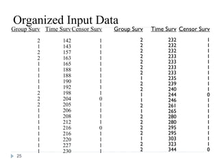
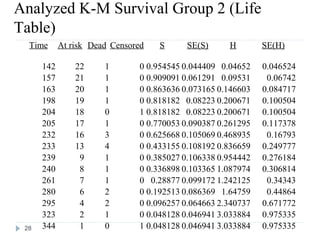
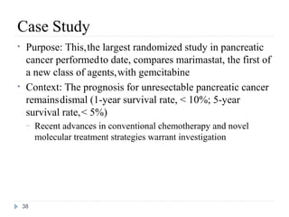
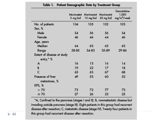
![Definition and Characteristics of Variables
Survival time (t) random variables (RVs) are always non-
negative, i.e., t ≥ 0.
T can either be discrete (taking a finite set of values, e.g.
a1, a2, …, an) or continuous [defined on (0,∞)].
A random variable t is called a censored survival time RV
if x = min(t, u), where u is a non-negative censoring
variable.
For a survival time RV, we need:
(1) an unambiguous time origin (e.g. randomization to clinical
trial)
(2) a time scale (e.g. real time (days, months, years)
(3) defnition of the event (e.g. death, relapse)
13](https://image.slidesharecdn.com/survcoxsardarpatelunivpart1final-130130010854-phpapp02/85/Part-1-Survival-Analysis-11-320.jpg)
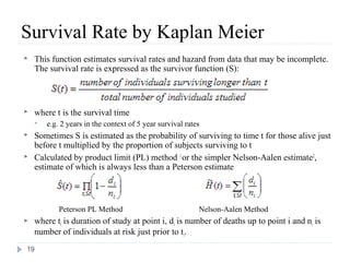
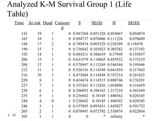
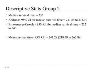

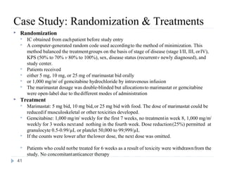
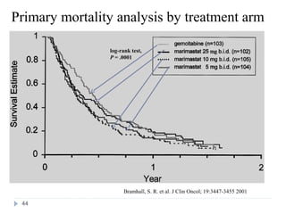
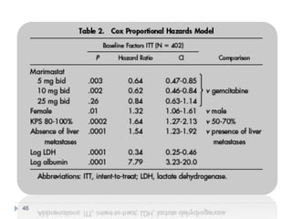
![Case Study: End Points
• The primary study end point
– Overall survival, along with prospectively defined comparisons
between gemcitabine and marimastat 25 mg bid and between
gemcitabine and marimastat 10 mg bid
– Secondary study end points
• Progression-free survival
• Patient benefit s
– quality of life [QOL], weight loss, pain, analgesic consumption, surgical
intervention to alleviate cancer symptoms, and KPS)
• Safety and tolerability
• Tumor response rate was also assessed
40](https://image.slidesharecdn.com/survcoxsardarpatelunivpart1final-130130010854-phpapp02/85/Part-1-Survival-Analysis-38-320.jpg)


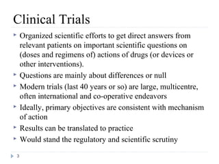
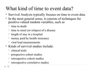
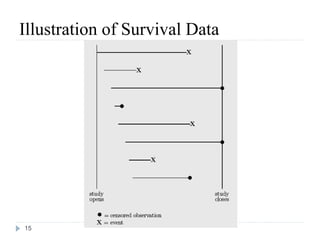
The document discusses survival analysis and Cox regression for cancer clinical trials. It begins with an overview of clinical trials for cancer, noting their complexity, long duration, high costs, and ethical concerns. It then covers survival analysis, describing key concepts like survival curves, hazard functions, and the Kaplan-Meier method for estimating survival when there is censoring. The document provides an example of survival data from a cancer study and discusses assumptions and parameters used in survival analysis like median and mean survival times.