Downloaded 505 times
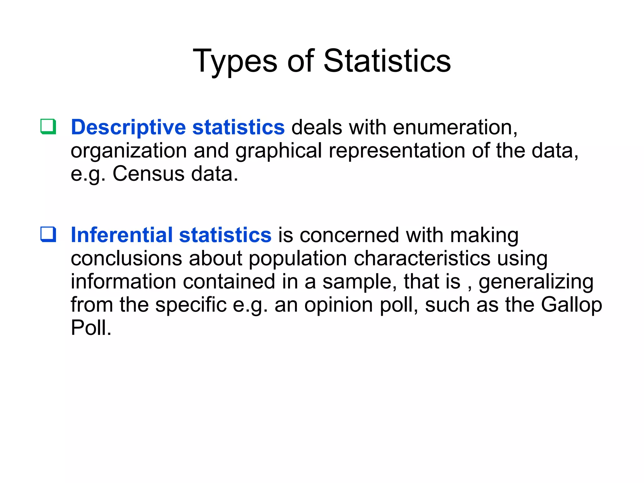


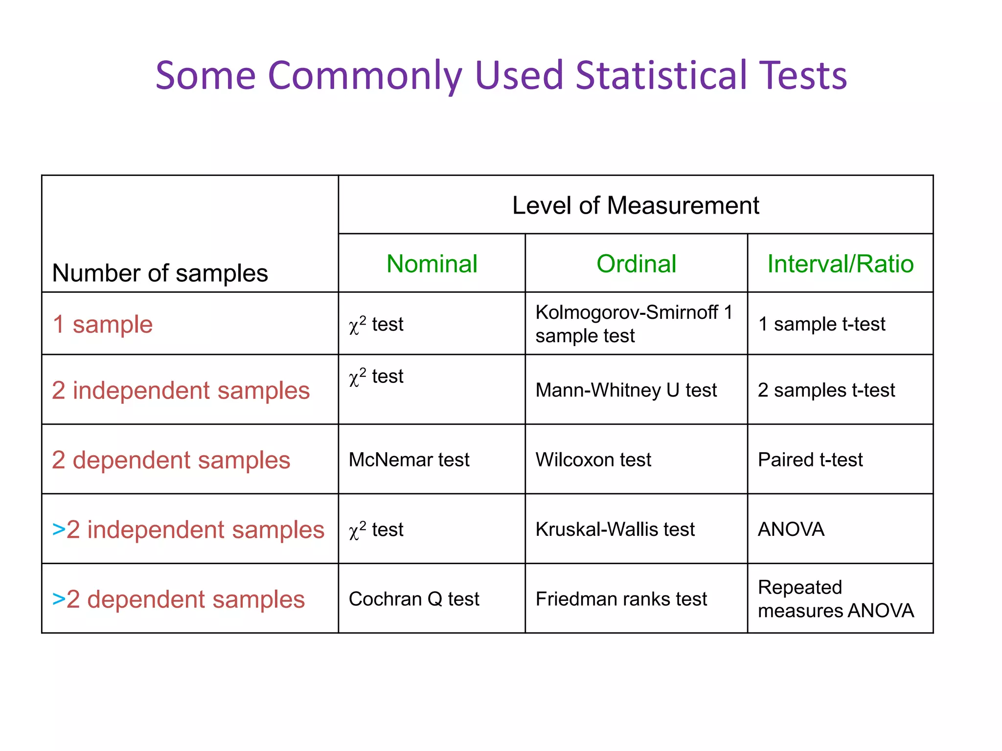


1) The document discusses commonly used statistical tests in research such as descriptive statistics, inferential statistics, hypothesis testing, and tests like t-tests, ANOVA, chi-square tests, and normal distributions. 2) It provides examples of how to determine sample sizes needed for adequate power in hypothesis testing and how to perform t-tests to analyze sample means. 3) Key statistical concepts covered include parameters, statistics, measurement scales, type I and II errors, and interpreting results of hypothesis tests.