This document provides an introduction to concepts in biostatistics and hypothesis testing. It outlines the objectives of learning about study design, types of data, hypothesis testing, p-values, and choosing appropriate statistical tests. It also describes office hours, topics beyond the scope of the class, and objectives for learning about stages of research studies, hypothesis tests, t-tests, and Wilcoxon tests.

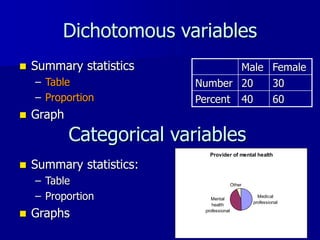
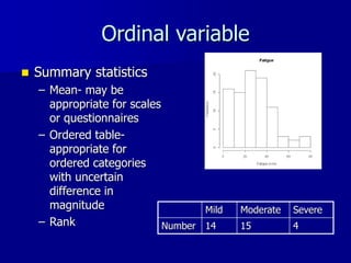
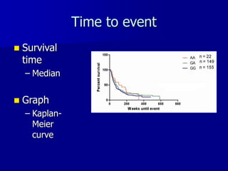
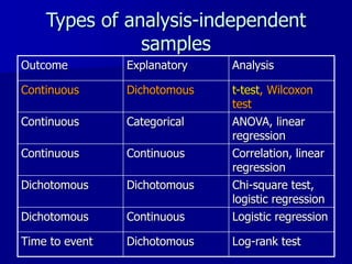
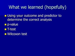
1. Introduction to
Biostatistics/Hypothesis
Testing
Brian Healy, PhD

2. Course objectives
 Introduction to concepts of biostatistics
– Type of data
– Hypothesis testing
– p-value
– Choosing the best statistical test
– Study design
– When you should get help
 Statistical thinking, not math proofs

3. Office hour
 Tuesday 9-11 in Room 2.140 of the
Simches building
 If you plan to come, please email me
(bchealy@partners.org) with a brief
description of your data so that I can
prepare

4. Beyond the scope
 Tutorial for a specific statistical package
– I will show output from some packages
(STATA, SAS, GraphPad)
 Topics that will be mentioned, but not
focused on
– Mixed models
– Principal components analysis
– ROC curves

5. Class objectives
 Introduction to biostatistics
– Stages of a research study
– Types of data
– Hypothesis test
– t-test
– Wilcoxon test
 Questions and requests for next time

6. Research study
I. Study design
• Experimental question- What are you trying to
learn? How will you prove this?
• Sample selection- Who are you going to study?
II. Data collection
• What should be collected?
III. Analysis of data
• Results- Was there any effect?
• Conclusions- What does this all mean? To whom
do results apply?

7. How is statistics related to each
stage?
I. Study design
• Experimental question- Define outcome, sources
of variability, unit and analysis plan
• Sample selection- Sample size, type of sample
II. Data collection
• What to collect?
III. Analysis of data
• Results- Hypothesis test
• Conclusion- Significance of effect/generalizability

8. Experimental question:
What? How?
Sample selection: Who? How many?
Collect Data
Analysis: Is there an effect?
Conclusion: To whom?

9. Example
 Multiple sclerosis is a progressive neurological
disorder
 We would like to find treatments that help
patients
 Unfortunately, it is very difficult to determine a
patient’s disease course because there are many
things going on
 How do we measure the change in the disease?
 What is the outcome?

11. Outcome variables
 An outcome variable is dependent
variable of interest
 The common outcome variables in MS
experiments are:
– Expanded disability status scale (EDSS)-
ordinal measure of disease severity
– Presence/absence of disease progression
– Expression a cytokine of interest (ex. IFN-g)
– Time to next relapse

12. Types of variables
 Continuous variable: Age, expression level
 Dichotomous variable: Dead/alive, Wild
type/mutant
 Categorical variable: Race, nominal scales
 Ordinal variable: Mild/Moderate/Severe,
level of stat knowledge
 Count outcomes: Number of lesions
 Time to event outcome: Time to death

13. Continuous variables
 Summary
statistics
– Location
 Mean
 Median
– Variability
 Standard
deviation
 Graphs

14. Dichotomous variables
 Summary statistics
– Table
– Proportion
 Graph
Male Female
Number 20 30
Percent 40 60
Categorical variables
 Summary statistics:
– Table
– Proportion
 Graphs
Provider of mental health
Medical
professional
Mental
health
professional
Other

15. Is this the correct interpretation?

16. Ordinal variable
 Summary statistics
– Mean- may be
appropriate for scales
or questionnaires
– Ordered table-
appropriate for
ordered categories
with uncertain
difference in
magnitude
– Rank
Mild Moderate Severe
Number 14 15 4

17. Time to event
 Survival
time
– Median
 Graph
– Kaplan-
Meier
curve

18. Description vs. comparison
 In many instances, description of the
outcome variable is the focus
– Estimate and confidence interval
 Based on results from survey, description
is not enough, rather comparison is of
interest
 What do we need for comparison?
– Second variable-usually called explanatory
variable

19. Explanatory variables
 Explanatory variables are the
independent variables that we believe
affect the outcome variables in some way
 In MS clinical studies, this can be
– Presence of disease
– Intervention/treatment (clinical trial)
– Genotype
– Expression of another cytokine
– Time

20. Types of analysis-independent
samples
Outcome Explanatory Analysis
Continuous Dichotomous t-test, Wilcoxon
test
Continuous Categorical ANOVA, linear
regression
Continuous Continuous Correlation, linear
regression
Dichotomous Dichotomous Chi-square test,
logistic regression
Dichotomous Continuous Logistic regression
Time to event Dichotomous Log-rank test

21. Comparison of two groups
 Question: Is the expression of CD-26 different in
relapsing MS patients compared to progressive
MS patients?
 What is the outcome?
– We measure CD-26 using flow cytometry
– Continuous variable
 What is the explanatory variable?
– Group membership (relapsing vs. progressive)
– Dichotomous variable
 How would you answer this question?
– Collect a sample from each group

22. Results
 Mean values:
– Relapsing patients=34.6
– Progressive patients=41.8
 The progressive patients had greater
production, but are we certain that there
is a difference between these?
– Statistically significant
– Clinically meaningful
 What is the variability in the data?

23.  Means in two
groups are
the same in
both
experiments
 Is there a
difference in
Experiment
1?
 In Experiment
2?
 Hypothesis
test
Experiment 1 Experiment 2

24. Reasons for differences between
groups
 Actual effect-when there is a difference
between the two groups
 Chance
 Bias
 Confounding
 Statistical tests are designed to determine
if the observed difference between the
groups was likely due to chance

25. Chance experiment
 Experiment: I flip a coin
– If heads, I win $1
– If tails, you win $1
 What if the following happened?
– 2 heads in a row
– 5 heads in a row
– 15 heads in a row
 Are you suspicious?

26. Null hypothesis
 In all experiments, we have an initial belief
– In coin example, you believed that there was a 50/50
chance of heads
 We always set up our null hypothesis so that we
can reject the null hypothesis.
 For our study, the null hypothesis is that the
mean in the relapsing MS patients is the same
as the mean in the progressive MS patients.

27. What is rare enough?
 This curve is the
distribution of the
statistic under the
null hypothesis
 If the observed
value is sufficiently
rare under the null,
we reject the null
hypothesis
 0.05 corresponds
to a 1 out of 20
chance
0.05
0.05

28. P-value
 Definition: the probability of the
observed result or something more
extreme under the null hypothesis
 If the probability of the event is
sufficiently small, we say that the
difference is likely not due simply to
chance and we have an actual effect.
 If p-value is small enough, we call the
effect statistically significant

29. What if p>0.05?
 In this case, the difference between the groups
is not statistically significant (at the 0.05 level).
 “If two values are not significantly different,
then by definition are they not identical?”
– No
– The two groups are not significantly different, but we
cannot say that they are the same
– We fail to reject the null hypothesis; we do not accept
that the null is true
– Bayesian statistics

30. Bias
 Is there
something in
my design
that led to my
result?

31. Steps for hypothesis testing
1) State null hypothesis
2) State type of data for explanatory and
outcome variable
3) Determine appropriate statistical test
4) State summary statistics if possible
5) Calculate p-value (stat package)
6) Decide whether to reject or not reject the null
hypothesis
• NEVER accept null
7) Write conclusion

32. Example
1) H0: meanrelapsing =meanprogressive
2) Explanatory: group membership-
dichotomous
Outcome: cytokine production-
continuous
• What test can we use to compare a
continuous outcome with a dichotomous
explanatory variable?

33. Two sample t-test
 A two sample t-test is a test for
differences in means in two samples.
 Assumption: Underlying population
distribution is normal
 The method of calculating the p-value is
beyond the scope of this class, but it is
easily found on-line
 Can get p-value from statistical package

34. Results
4) meanrelapsing =34.6, meanprogressive=41.8
5) Calculate p-value:
Two Sample t-test
t = -1.19, df = 22.8, p-value = 0.25
95 percent confidence interval: (-5.3, 19.7)
6) Fail to reject the null hypothesis because p-
value is less than 0.05
7) Conclusion: The difference between the
groups is not statistically significant.

35. p-value
summary statistics

36. summary statistics
p-value

37.  Significant
difference in
experiment 1
 Added
variance in
experiment 2
led to non-
significant
result
 What does
this mean?
Experiment 1 Experiment 2
p<0.0001
p=0.25

38. Types of analysis-independent
samples
Outcome Explanatory Analysis
Continuous Dichotomous t-test, Wilcoxon
test
Continuous Categorical ANOVA, linear
regression
Continuous Continuous Correlation, linear
regression
Dichotomous Dichotomous Chi-square test,
logistic regression
Dichotomous Continuous Logistic regression
Time to event Dichotomous Log-rank test

39. Example
 Experimental Autoimmune Encephalomyelitis
(EAE) in mice is the animal model for multiple
sclerosis (MS)
 The effect of various interventions are first
tested in mice
 A common hypothesis is that treating mice with
a specific intervention will either inhibit or
promote the disease
 How do we measure the change in the disease?
 What is the outcome?

40. Monkey wrench
 What if
underlying data
is not normal?
 An outcome in
an EAE study is
the disease
grade, which is
an ordinal scale
Disease severity scores
0
1
2
3
4
5
6
7
0 1 2 3 4
Score
Frequency
KO
Wild-type

41. Wilcoxon rank sum test
 Wilcoxon rank sum test is a nonparametric
test that allows group comparison if
– Ordinal data
– Rank data
– Underlying data are non-normal
– Outliers
 Steps for hypothesis test using a Wilcoxon
test are exactly the same

42. Hypothesis test
1) H0: medianKO =medianWild type
2) Predictor: dichotomous
Outcome: ordinal
3) Test: Wilcoxon rank sum test
4) MedianKO=1; MedianWild type=2
5) Calculate p-value: p = 0.19
6) Fail to reject null hypothesis
7) There is not significant evidence of a
difference between the two groups

43. p-value

44. Dependent observations
 Up to now we have assumed that observations
are independent
 What if we have related observations?
– On and off treatment on the same subject
– Left and right eye from the same subject
– Multiple observations over time
 The big advantage of dependent observations is
the same subject is observed under multiple
conditions
 Independent tests fail to account for correlation

45. Example
 In MS patients, the intensity of areas of
the brain on T1-weighted MRI are of
interest to determine if there is damage
 In particular, the intensity of the putamen
of left and right side of the brain was
measured in 35 MS patients
 We believed that there would be more
significant hypointensity in the left side

46.  There may a
difference
between the
groups
 Are we
interested
just in the
mean at
each time
point?

47.  The
difference
between the
time points
is the
outcome
 Is the
difference
significantly
different
from 0?

48. Hypothesis test
1) H0: meanleft=meanright
2) Paired continuous data with side as
explanatory variable
3) Paired t-test
4) Mean difference=0.063
5) p-value=0.046
6) Since the p-value is less than 0.05, we can
reject the null hypothesis
7) We conclude that the intensity is unequal in
the two sides of the brain

49. p-value

50. Types of analysis-dependent
samples
Outcome Predictor Analysis
Continuous Dichotomous Paired t-test,
Wilcoxon signed
rank test
Continuous Categorical Repeated
measures ANOVA
Continuous Continuous Mixed model
Dichotomous Dichotomous McNemar’s test
Dichotomous Continuous Repeated
measures logistic
regression

51. Other dependent samples
 Continuous outcome/categorical
explanatory variable
– Subject is measured under three conditions
– Subject is measures at three time points

52.  Each dot
represents an
observation
for a mouse
at each of the
markers
 There was a
negative
control in this
experiment
(Group = 0)

53. What should we do?
 What is the hypothesis?
– Is the expression of any of the markers
different than the control?
 Repeated measures ANOVA/mixed model
– Can proceed with normal hypothesis test
 Must always think about assumptions of
model
– Do we have equal variance?
 Consult a statistician

54. Why use dependent samples?
 Sometimes it is required based on the
study
 Often can increase power depending on
the outcome because one major source of
variability is accounted for
– Changes over time
 Consult a statistician if you want to
determine the best study design

55. Helpful website
 http://www.ats.ucla.edu/stat/stata/whatst
at/default.htm
 Shows how to complete many of these
analyses in various statistical packages

56. What we learned (hopefully)
 Using your outcome and predictor to
determine the correct analysis
 p-value
 T-test
 Wilcoxon test