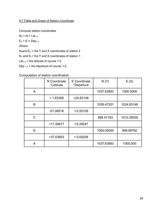
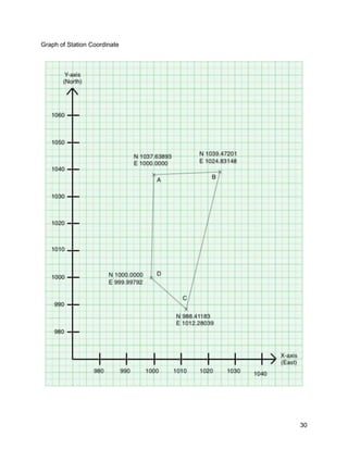
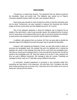
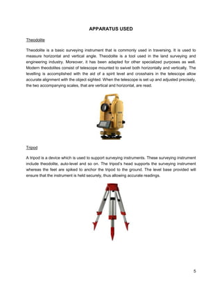
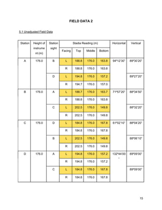
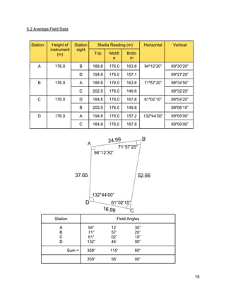
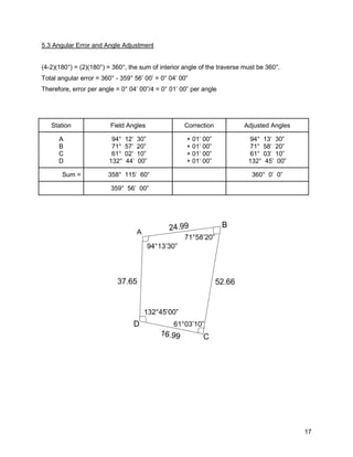
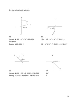
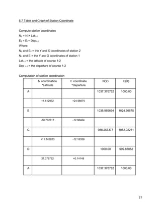
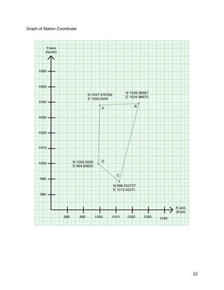
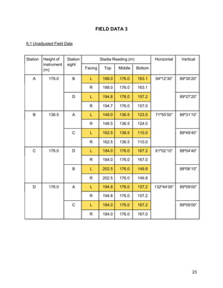
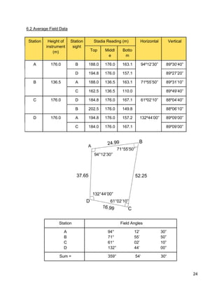
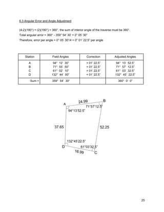
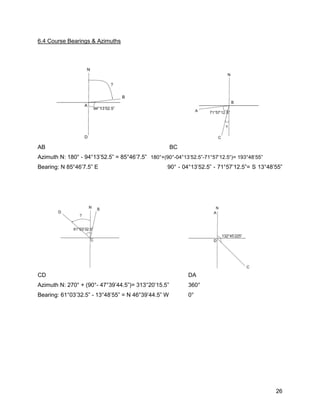
This document is a field report for a traversing survey conducted by students. It contains unadjusted and average field data from three separate traverses, including measured horizontal and vertical angles between stations. It also shows the calculations to determine angular errors, angle adjustments, course bearings, latitudes and departures, adjusted coordinates, and station positions. The objectives, equipment used, and results are presented in tables and graphs.

1. SCHOOL OF ARCHITECTURE, BUILDING AND
DESIGN
BACHELOR OF QUANTITY SURVEYING (HONOURS)
SITE SURVEYING [QSB 60103]
FIELD WORK 2 REPORT
TRAVERSING
DARREN TAN QUAN WEN 0322662
YEAP PHAY SHIAN 0322243
LEE XIN YING 0322432
MICHELLE TUNG MAN KAYE 0324175
LOH MUN TONG 0323680
LECTURER: MR. CHAI VOON CHIET
SUBMISSION DATE: 8th DECEMBER 2016

2. 1
TABLE OF CONTENT
NO. TOPIC PAGE
1. INTRODUCTION TO TRAVERSING 2 - 3
2. OBJECTIVES 4
3. APPARATUS USED 5 - 6
4. FIELD DATA 1
4.1 Unadjusted Field Data
4.2 Average Field Data
4.3 Angular error and angle adjustment
4.4 Course Bearings & Azimuths
4.5 Course Latitudes & Departures
4.6 Adjusted Latitudes & Departures
4.7 Table and Graph of Station Coordinate
7 - 14
5. FIELD DATA 2
5.1 Unadjusted Field Data
5.2 Average Field Data
5.3 Angular error and angle adjustment
5.4 Course Bearings & Azimuths
5.5 Course Latitudes & Departures
5.6 Adjusted Latitudes & Departures
5.7 Table and Graph of Station Coordinate
15 - 22
6. FIELD DATA 3
6.1 Unadjusted Field Data
6.2 Average Field Data
6.3 Angular error and angle adjustment
6.4 Course Bearings & Azimuths
6.5 Course Latitudes & Departures
6.6 Adjusted Latitudes & Departures
6.7 Table and Graph of Station Coordinate
23 - 30
9. DISCUSSION 31

3. 2
INTRODUCTION TO TRAVERSING
A traverse survey involves a connected sequence of lines whose length and directions
are measured. It is perhaps the most common type of control survey performed by surveyors in
private practice or employed by local government agencies. Precise traverse surveys are much
more practical nowadays with the use of electronic distance measuring (EDM) devices.
Traversing is a type of survey in which a number of connected survey lines from the
framework and the directions and lengths of the survey lines are measured with the help of an
angle measuring instrument and a tape or chain respectively. The angles are measured using
theodolites, or total stations, whereas the distances can be measured using total stations, steel
tapes or electronic distance-measurement instruments (EDMs).
There are two types of traverse:
(1) Open traverse: When the lines from a circuit ends elsewhere
(2) Closed traverse: When the lines from a circuit which ends at the starting point

4. 3
(1) Open traverse
An open traverse is a series of measured straight lines that do not intersect or form a loop. This
lack of geometric closure means that there is no geometric verification possible with respect to
the actual positioning of the traverse stations. In route surveys, open traverse station positioning
can be verified by computation from available tied-in field markers as shown on property plans,
or through the use of global positioning system (GPS) receivers.
(2) Closed traverse
A closed traverse is connected lines that start at a point and ends at the same point or at a point
whose relative position is known. The errors during measurement are minimized and adjusted to
get accurate data. Closed traverse is the primary method used in checking surveying field work.
There are two types of closed traverse:
(a) Loop traverse – A loop traverse starts and ends at the same point, forming a closed
geometric figure called a polygon.
(b) Connecting traverse – A connecting traverse looks like an open traverse, however
the only difference is, it begins and ends at points (or lines) of
known position (and direction) at each end of the traverse.

5. 4
OBJECTIVES
● To enhance a better understanding of the traverse process.
● To determine the area encompassed within a boundary.
● To determine the angular error and closing error of traverse conducted.
● To make necessary adjustments in obtaining an accurate data.
● To experience the life of being as a Quantity Surveyor and experience the actual
working environment.
● To help them to understand the correct way to read the reading on the theodolite
and record the data.
● To give the students a chance to familiarize with the actual working atmosphere
on the site including uncertainty situations.
● To provide them the opportunity of hands on experience of setting up the
theodolite for angle measurements.

6. 5
APPARATUS USED
Theodolite
Theodolite is a basic surveying instrument that is commonly used in traversing. It is used to
measure horizontal and vertical angle. Theodolite is a tool used in the land surveying and
engineering industry. Moreover, it has been adapted for other specialized purposes as well.
Modern theodolites consist of telescope mounted to swivel both horizontally and vertically. The
levelling is accomplished with the aid of a spirit level and crosshairs in the telescope allow
accurate alignment with the object sighted. When the telescope is set up and adjusted precisely,
the two accompanying scales, that are vertical and horizontal, are read.
Tripod
A tripod is a device which is used to support surveying instruments. These surveying instrument
include theodolite, auto-level and so on. The tripod’s head supports the surveying instrument
whereas the feet are spiked to anchor the tripod to the ground. The level base provided will
ensure that the instrument is held securely, thus allowing accurate readings.

7. 6
Plumb bob
A plumb bob or a plummet is a weight with a pointed tip on the bottom that is suspended from a
string and used as a vertical reference line. This instrument used in surveying to sight a point on
the ground that is not readily visible. They are used to set the instrument exactly over a fixed
datum marker, prior to taking fresh readings.
Levelling Staff
The levelling staff is simply a large ruler, available in lengths of 3, 4, or 5 metres and usually
made of aluminium with telescopic sections. The levelling staff is sectional so that can be
adjusted in length to allow for easy storage and transport. The sections have locking buttons to
ensure accurate length is maintained.
The “E” pattern is designed to make it easy to read a small section of the scale when see
through a telescope.

8. 7
FIELD DATA 1
4.1 Unadjusted Field Data
Station Height of
instrume
nt (m)
Station
sight
Stadia Reading (m) Horizontal Vertical
Facing Top Middle Bottom
A 131.0 B L 143.2 131.0 118.5 94º18’00” 90º28’40”
R 143.2 131.0 118.0
D L 149.5 131.0 112.0 90º06’10”
R 149.5 131.0 112.0
B 125.0 A L 137.0 125.0 112.0 71º55’50” 89º30’50”
R 137.5 125.0 112.5
C L 151.0 125.0 99.0 89º56’50”
R 151.0 125.0 99.0
C 176.0 D L 184.5 176.0 167.5 61º01’40” 88º04’30”
R 184.5 176.0 167.5
B L 202.0 176.0 149.5 89º33’00”
R 202.0 176.0 149.5
D 176.0 A L 194.5 176.0 157.0 134º22’50
”
89º13’30”
R 194.5 176.0 157.0
C L 184.5 176.0 167.5 88º51’20”
R 184.5 176.0 167.5

9. 8
4.2 Average Field Data
Station Height of
instrument
(m)
Station
sight
Stadia Reading (m) Horizontal Vertical
Top Middl
e
Botto
m
A 131.0 B 143.2 131.0 118.3 94º18’00” 90º28’40”
D 149.5 131.0 112.0 90º06’10”
B 125.0 A 137.3 125.0 112.3 71º55’50” 89º30’50”
C 151.0 125.0 99.0 89º56’50”
C 176.0 D 184.5 176.0 167.5 61º01’40” 88º04’30”
B 202.0 176.0 149.5 89º33’00”
D 176.0 A 194.5 176.0 157.0 134º22’50” 89º13’30”
C 184.5 176.0 167.5 88º51’20”
Station Field Angles
A
B
C
D
94° 18’ 00”
71° 55’ 50”
61° 01’ 40”
134° 22’ 50”
Sum = 360° 96‘ 140“
361° 38’ 20”

10. 9
4.3 Angular Error and Angle Adjustment
(4-2)(180°) = (2)(180°) = 360°, the sum of interior angle of the traverse must be 360°.
Total angular error = 360° - 361° 38’ 20’ = -1° 38’ 20”
Therefore, error per angle = -1° 38’ 20”/4 = -5900”/4 = -24’ 35” per angle
Station Field Angles Correction Adjusted Angles
A
B
C
D
94° 18’ 00”
71° 55’ 50”
61° 01’ 40”
134° 22’ 50”
- 24’ 35”
- 24’ 35”
- 24’ 35”
- 24’ 35”
93° 53’ 25”
71° 31’ 15”
60° 37’ 05”
133° 58’ 15”
Sum = 360° 96‘ 140“ 360° 0’ 0”
361° 38’ 20”

11. 10
4.4 Course Bearings & Azimuths
AB BC
Azimuth N: 180° - 93°53’25” = 86°06’35” 180° + (90° - 03°53’25” - 71°31‘15“) =
194°35’20”
Bearing: N 86°06’35” E 90° - 03°53’25” - 71°31’15” = S 14°35’20” W
CD DA
Azimuth N: 270° + (90°- 46°01’45”) = 313°58’15” 360°
Bearing: 60°37’05” - 14°35’20” = N 46°01’45” W 0°

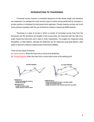
12. 11
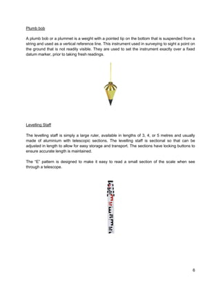
4.5 Course Latitudes & Departures
Cos β Sin β L cosβ L sinβ
Station Bearing, β Length, L Cosine Sine Latitude Departure
A
B
C
D
A
N 86°06’35” E
S 14°35’20” W
N 46°01’45” W
0°
24.950
52.250
16.990
37.495
0.0678
0.9678
0.6943
1.000
0.9977
0.2519
0.7197
0.000
+ 1.69161
- 50.56755
+ 11.79620
+ 37.49500
+ 24.8926
- 13.1618
- 12.2277
0.0000
Sum = 131.685 + 0.41526 - 0.4969
Accuracy = 1: (P/Ec)
For average land surveying, an accuracy is typically about 1:3000.
Ec = [(Error in Latitude)2
+ (Error in Departure)2
] 1/2
= [(0.41526)
2
+ (-0.4969)
2
]
1/2
= 0.6476
P = 131.685
Accuracy = 1: (131.685 / 0.6478)
= 1: 203.28
∴ The traversing is not acceptable.

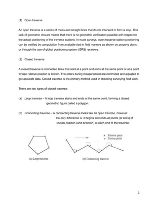
13. 12
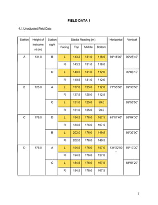
4.6 Adjusted Latitudes & Departures
The Compass Rule
Correction = – [∑∆y] / P × L or – [∑∆x] / P × L
Where
∑∆y and ∑∆x = the error in latitude or in departure
P = the total length or perimeter of the traverse
L = the length of a particular course
Compass rule correction to latitude and departure
Unadjusted Correction Adjusted
Latitude Departure Latitude Departure Latitude Departure
A
+1.8418 +24.9225 0.0214 0.02230 +1.8632 +24.9448
B
-51.1381 -12.5647 0.0452 0.04697 -51.0929 -12.51773
C
+11.5328 -12.4758 0.0146 0.01515 +11.5474 -12.46065
D
+37.65 0 0.0323 0.03358 +37.6823 +0.03358
A
-0.1135 -0.118 0.1135 0.118 0.0 0.0
Check Check

14. 13
4.7 Table and Graph of Station Coordinate
Compute station coordinates
N2 = N1+ Lat1-2
E2 = E1+ Dep1-2
Where
N2 and E2 = the Y and X coordinates of station 2
N1 and E1= the Y and X coordinates of station 1
Lat1-2 = the latitude of course 1-2
Dep 1-2 = the departure of course 1-2
Computation of station coordination
N coordination
*Latitude
E coordinate
*Departure
N(Y) E(X)
A 1037.6823 1000.00
+1.8632 +24.9448
B 1039.5455 1024.9448
-51.0929 -12.51773
C 988.4526 1012.42707
+11.5474 -12.46065
D 1000.00 999.96642
+37.6823 +0.03358
A 1037.0823 1000.00

15. 14
Graph of Station Coordinate

16. 15
FIELD DATA 2
5.1 Unadjusted Field Data
Station Height of
instrume
nt (m)
Station
sight
Stadia Reading (m) Horizontal Vertical
Facing Top Middle Bottom
A 176.0 B L 188.8 176.0 163.8 94º12’30” 89º30’20”
R 188.8 176.0 163.8
D L 194.8 176.0 157.2 89º27’20”
R 194.7 176.0 157.0
B 176.0 A L 188.7 176.0 163.7 71º57’20” 88º34’50”
R 188.8 176.0 163.8
C L 202.5 176.0 149.8 88º32’20”
R 202.5 176.0 149.8
C 176.0 D L 184.8 176.0 167.8 61º02’10” 88º04’20”
R 184.8 176.0 167.8
B L 202.5 176.0 149.8 88º06’10”
R 202.5 176.0 149.8
D 176.0 A L 194.8 176.0 157.2 132º44’00
”
89º09’00”
R 194.8 176.0 157.2
C L 184.8 176.0 167.8 89º09’00”
R 184.8 176.0 167.8

17. 16
5.2 Average Field Data
Station Height of
instrument
(m)
Station
sight
Stadia Reading (m) Horizontal Vertical
Top Middl
e
Botto
m
A 176.0 B 188.8 176.0 163.8 94º12’30” 89º30’20”
D 194.8 176.0 157.1 89º27’20”
B 176.0 A 188.8 176.0 163.8 71º57’20” 88º34’50”
C 202.5 176.0 149.8 88º32’20”
C 176.0 D 184.8 176.0 167.8 61º02’10” 88º04’20”
B 202.5 176.0 149.8 88º06’10”
D 176.0 A 194.8 176.0 157.2 132º44’00” 89º09’00”
C 184.8 176.0 167.8 89º09’00”
Station Field Angles
A
B
C
D
94° 12’ 30”
71° 57’ 20”
61° 02’ 10”
132° 44’ 00”
Sum = 358° 115‘ 60“
359° 56’ 00”

18. 17
5.3 Angular Error and Angle Adjustment
(4-2)(180°) = (2)(180°) = 360°, the sum of interior angle of the traverse must be 360°.
Total angular error = 360° - 359° 56’ 00’ = 0° 04’ 00”
Therefore, error per angle = 0° 04’ 00”/4 = 0° 01’ 00” per angle
Station Field Angles Correction Adjusted Angles
A
B
C
D
94° 12’ 30”
71° 57’ 20”
61° 02’ 10”
132° 44’ 00”
+ 01’ 00”
+ 01’ 00”
+ 01’ 00”
+ 01’ 00”
94° 13’ 30”
71° 58’ 20”
61° 03’ 10”
132° 45’ 00”
Sum = 358° 115‘ 60“ 360° 0’ 0”
359° 56’ 00”

19. 18
5.4 Course Bearings & Azimuths
AB BC
Azimuth N: 180° - 94°13’30” = 85°46’30” 180° + (90° - 04°13’30” - 71°58’20”) =
193°48’10”
Bearing: N 85°46’30” E 90° - 03°53’25” - 71°58’20” = S 13°48’10”
CD DA
Azimuth N: 270° + (90°- 47°15’00”) = 312°45’00” 360°
Bearing: 61°03’10” - 13°48’10” = N 47°15’00” W 0°

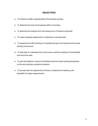
20. 19
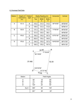
5.5 Course Latitudes & Departures
Cos β Sin β L cosβ L sinβ
Station Bearing, β Length, L Cosine Sine Latitude Departure
A
B
C
D
A
N 85°46’30” E
S 13°48’10” W
N 47°15’00” W
0°
24.990
52.660
16.990
37.650
0.0737
0.9711
0.6788
1.000
0.9973
0.2386
0.7343
0.000
+ 1.8418
- 51.1381
+ 11.5328
+ 37.650
+ 24.9225
- 12.5647
- 12.4758
0.0000
Sum = 132.290 - 0.1135 - 0.1180
Accuracy = 1: (P/Ec)
For average land surveying, an accuracy is typically about 1:3000.
Ec = [(Error in Latitude)2
+ (Error in Departure)2
] 1/2
= [(-0.1135)
2
+ (-0.1180)
2
]
1/2
= 0.1637
P = 132.290
Accuracy = 1: (132.290 / 0.1637)
= 1: 808.12
∴ The traversing is not acceptable.

21. 20
5.6 Adjusted Latitudes & Departures
The Compass Rule
Correction = – [∑∆y] / P × L or – [∑∆x] / P × L
Where
∑∆y and ∑∆x = the error in latitude or in departure
P = the total length or perimeter of the traverse
L = the length of a particular course
Compass rule correction to latitude and departure
Unadjusted Correction Adjusted
Latitude Departure Latitude Departure Latitude Departure
A
+1.69161 +24.8926 -0.078678 0.09415 +1.612932 +24.98675
B
-50.56755 -13.1618 -0.164767 0.19716 -50.732317 -12.96464
C
+11.7962 -12.2277 -0.053577 0.06411 +11.74262
3
-12.16359
D
+37.495 0 -0.118238 0.14148 +37.37676
2
+0.14148
A
0.41526 -0.4969 -0.41526 0.4969 0.0 0.0
Check Check

22. 21
5.7 Table and Graph of Station Coordinate
Compute station coordinates
N2 = N1+ Lat1-2
E2 = E1+ Dep1-2
Where
N2 and E2 = the Y and X coordinates of station 2
N1 and E1= the Y and X coordinates of station 1
Lat1-2 = the latitude of course 1-2
Dep 1-2 = the departure of course 1-2
Computation of station coordination
N coordination
*Latitude
E coordinate
*Departure
N(Y) E(X)
A 1037.376762 1000.00
+1.612932 +24.98675
B 1038.989694 1024.98675
-50.732317 -12.96464
C 988.257377 1012.02211
+11.742623 -12.16359
D 1000.00 999.85852
37.376762 +0.14148
A 1037.376762 1000.00

23. 22
Graph of Station Coordinate

24. 23
FIELD DATA 3
6.1 Unadjusted Field Data
Station Height of
instrument
(m)
Station
sight
Stadia Reading (m) Horizontal Vertical
Facing Top Middle Bottom
A 176.0 B L 188.0 176.0 163.1 94º12’30” 89º30’20”
R 188.0 176.0 163.1
D L 194.8 176.0 157.2 89º27’20”
R 194.7 176.0 157.0
B 136.5 A L 149.0 136.5 123.5 71º55’50” 89º31’10”
R 148.5 136.5 124.0
C L 162.5 136.5 110.0 89º49’40”
R 162.5 136.5 110.0
C 176.0 D L 184.0 176.0 167.2 61º02’10” 88º04’40”
R 184.0 176.0 167.0
B L 202.5 176.0 149.8 88º06’10”
R 202.5 176.0 149.8
D 176.0 A L 194.8 176.0 157.2 132º44’00” 89º09’00”
R 194.8 176.0 157.2
C L 184.0 176.0 167.2 89º09’00”
R 184.0 176.0 167.0

25. 24
6.2 Average Field Data
Station Height of
instrument
(m)
Station
sight
Stadia Reading (m) Horizontal Vertical
Top Middl
e
Botto
m
A 176.0 B 188.0 176.0 163.1 94º12’30” 89º30’40”
D 194.8 176.0 157.1 89º27’20”
B 136.5 A 188.0 136.5 163.1 71º55’50” 89º31’10”
C 162.5 136.5 110.0 89º49’40”
C 176.0 D 184.8 176.0 167.1 61º02’10” 88º04’40”
B 202.5 176.0 149.8 88º06’10”
D 176.0 A 194.8 176.0 157.2 132º44’00” 89º09’00”
C 184.0 176.0 167.1 89º09’00”
Station Field Angles
A
B
C
D
94° 12’ 30”
71° 55’ 50”
61° 02’ 10”
132° 44’ 00”
Sum = 359° 54‘ 30“

26. 25
6.3 Angular Error and Angle Adjustment
(4-2)(180°) = (2)(180°) = 360°, the sum of interior angle of the traverse must be 360°.
Total angular error = 360° - 359° 54’ 30’ = 0° 05’ 30”
Therefore, error per angle = 0° 05’ 30”/4 = 0° 01’ 22.5” per angle
Station Field Angles Correction Adjusted Angles
A
B
C
D
94° 12’ 30”
71° 55’ 50”
61° 02’ 10”
132° 44’ 00”
+ 01’ 22.5”
+ 01’ 22.5”
+ 01’ 22.5”
+ 01’ 22.5”
94° 13’ 52.5”
71° 57’ 12.5”
61° 03’ 32.5”
132° 45’ 22.5”
Sum = 359° 54‘ 30“ 360° 0’ 0”

27. 26
6.4 Course Bearings & Azimuths
AB BC
Azimuth N: 180° - 94°13’52.5” = 85°46’7.5” 180°+(90°-04°13’52.5”-71°57‘12.5“)= 193°48’55”
Bearing: N 85°46’7.5” E 90° - 04°13’52.5” - 71°57’12.5”= S 13°48’55”
CD DA
Azimuth N: 270° + (90°- 47°39’44.5”)= 313°20’15.5” 360°
Bearing: 61°03’32.5” - 13°48’55” = N 46°39’44.5” W 0°

28. 27
6.5 Course Latitudes & Departures
Cos β Sin β L cosβ L sinβ
Station Bearing, β Length, L Cosine Sine Latitude Departure
A
B
C
D
A
N 85°46’7.5” E
S 13°48’55” W
N 46°39’44.5”
W
0°
24.898
52.571
16.889
37.645
0.0738
0.9711
0.6863
1.000
0.9973
0.2388
0.7273
0.000
+ 1.8371
- 51.0517
+ 11.5909
+ 37.6450
+ 24.8301
- 12.5540
- 12.2834
0.0000
Sum = 132.003 0.0213 - 0.0073
Accuracy = 1: (P/Ec)
For average land surveying, accuracy is typically about 1:3000.
Ec = [(Error in Latitude) 2
+ (Error in Departure) 2
] 1/2
= [(0.0213) 2
+ (- 0.0073) 2
] 1/2
= 0.0225
P = 132.003
Accuracy = 1: (132.003 / 0.0225)
= 1: 5866.80
∴ The traversing is acceptable.

29. 28
6.6 Adjusted Latitudes & Departures
The Compass Rule
Correction = – [∑∆y] / P × L or – [∑∆x] / P × L
Where
∑∆y and ∑∆x = the error in latitude or in departure
P = the total length or perimeter of the traverse
L = the length of a particular course
Correction to latitude and departure
Unadjusted Correction Adjusted
Latitude Departure Latitude Departure Latitude Departure
A
+ 1.8371 + 24.8301 -0.00402 + 0.00138 + 1.83308 +24.83148
B
-51.0517 -12.5540 - 0.00848 + 0.00291 -51.06018 -12.55109
C
+ 11.5909 -12.2834 - 0.00273 + 0.00093 +11.58817 -12.28247
D
+ 37.6450 0.0000 - 0.00607 + 0.00208 +37.63893 + 0.00208
A
+ 0.0213 - 0.0073 - 0.02130 + 0.00730 0.0000 0.0000
Checked Checked

30. 29
6.7 Table and Graph of Station Coordinate
Compute station coordinates
N2 = N1+ Lat1-2
E2 = E1+ Dep1-2
Where
N2and E2 = the Y and X coordinates of station 2
N1 and E1= the Y and X coordinates of station 1
Lat1-2 = the latitude of course 1-2
Dep 1-2 = the departure of course 1-2
Computation of station coordination
N Coordinate
*Latitude
E Coordinate
*Departure
N (Y) E (X)
A 1037.63893 1000.0000
+ 1.83308 +24.83148
B 1039.47201 1024.83148
-51.06018 -12.55109
C 988.41183 1012.28039
+11.58817 -12.28247
D 1000.00000 999.99792
+37.63893 + 0.00208
A 1037.63893 1000.000

31. 30
Graph of Station Coordinate

32. 31
DISCUSSION
Traversing is a closed loop traverse. The equipment that we utilized overall are
the theodolite, tripod and plumb bob. The fieldwork was carried out at Taylor’s
University Lakeside Campus staff’s car park, near Academic Block E.
Each group was required to mark at least four points so that the traversing work
can be done. Furthermore, we were required to measure the horizontal and vertical
angles at the four points which are then labelled as point A, B, C and D.
One of the apparent obstacles in doing the fieldwork was to balance the air
bubble in the spirit level in order to get accurate results. We realised that the 5 person
count in each group is the optimal head-count to get our job done quickly and smoothly,
as each person was assigned to one specific task throughout the fieldwork.
In addition, with guidance from our lecturer, Mr Chai, we were able to identify the
important steps of the fieldwork and also the proper way to operate the theodolite.
However, after repeating the fieldwork 2 times, we were still unable to obtain an
accurate and acceptable result. We realised that even the slightest error in taking the
readings can result in final readings that stray off too much from the acceptable error.
We took our second set of readings which is more accurate than the first set, but still not
closed to the acceptable error. Mr. Chai then asked us to do the 3rd time, however this
time we used a different instrument. We manage to take all 4 points. Thankfully we
managed to close it with our 3rd data after using a different instrument.
In conclusion, practical experience in surveying is very important aside from
everything we have learnt in the classroom. We also learn that 3 problems will arise
when doing traversing such as human error, instrument error and random error such as
heavy rain, strong wind and others.