This document provides details on a closed traverse survey conducted by students. It includes:
1. An introduction to traverse surveys and the different types of traverses.
2. Details of the fieldwork including measured angles, distances, bearings, latitudes and departures.
3. Calculations to adjust the measured values including distributing angular error, computing horizontal and vertical distances, and determining error of closure.
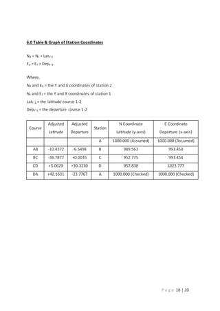
4. Presentation of the adjusted course latitudes and departures, showing an improved closure with errors of 0.0281m in latitude and 0.001m in departure.


![P a g e 11 | 20
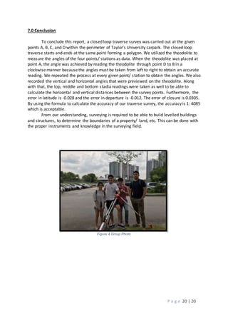
Top Stadia : 1.857
Bottom Stadia : 1.735
Top Stadia : 1.856
Bottom Stadia : 1.735
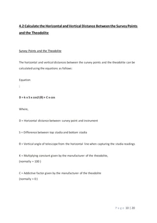
Distance A-B = [ (K x s x Cos² θ) + ( C x Cos θ )
= [ 100 x (1.857-1.735) 0.9971 ] + (0 x Cos θ)
= 12.165m
Top Stadia : 1.859
Bottom Stadia : 1.735
Top Stadia : 1.860
Bottom Stadia : 1.735
Distance B-A = [ (K x s x Cos² θ) + ( C x Cos θ )
= [ 100 x (1.860-1.735) 0.9988 ] + (0 x Cos θ)
= 12.485m
Top Stadia : 1.988
Bottom Stadia : 1.623
Top Stadia : 1.989
Bottom Stadia : 1.623
Distance B-C = [ (K x s x Cos² θ) + ( C x Cos θ )
= [ 100 x (1.989-1.623) 0.9999 ] + (0 x Cos θ)
= 36.596m
Top Stadia : 1.993
Bottom Stadia : 1.624
Top Stadia : 1.994
Bottom Stadia : 1.624
Distance C-B = [ (K x s x Cos² θ) + ( C x Cos θ )
= [ 100 x (1.994-1.624) 0.9999 ] + (0 x Cos θ)
= 36.996m](https://image.slidesharecdn.com/sitesurveyreport2-171221190515/85/Site-survey-report-2-11-320.jpg)
![P a g e 12 | 20
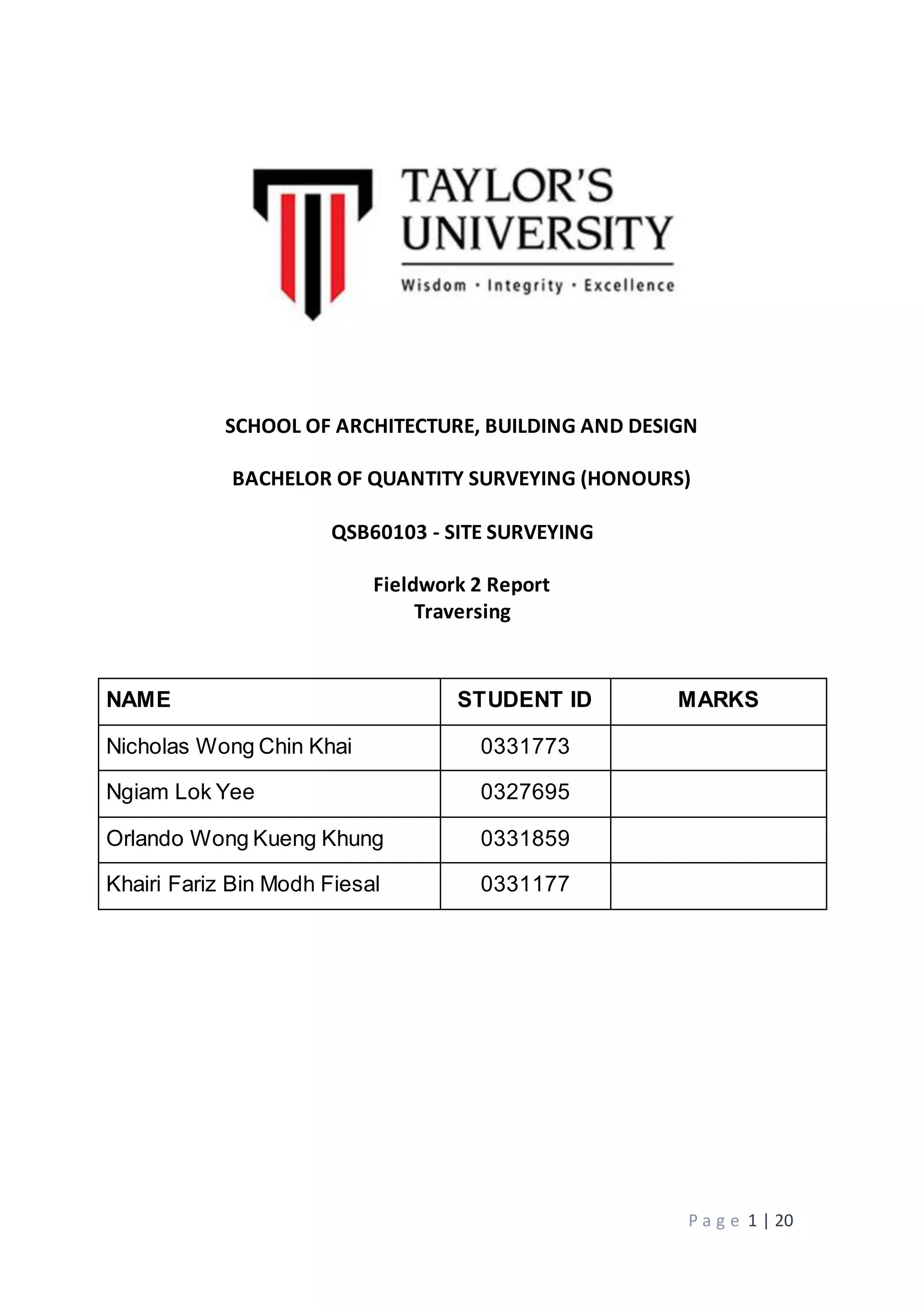
Top Stadia : 1.994
Bottom Stadia : 1.685
Top Stadia : 1.995
Bottom Stadia : 1.685
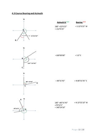
Distance C-D = [ (K x s x Cos² θ) + ( C x Cos θ )
= [ 100 x (1.995-1.685) 0.9996 ] + (0 x Cos θ)
= 30.988m
Top Stadia : 1.990
Bottom Stadia : 1.685
Top Stadia : 1.990
Bottom Stadia : 1.684
Distance D-C = [ (K x s x Cos² θ) + ( C x Cos θ )
= [ 100 x (1.990-1.685) 0.9996 ] + (0 x Cos θ)
= 30.488m
Top Stadia : 2.019
Bottom Stadia : 1.573
Top Stadia : 2.019
Bottom Stadia : 1.573
Distance D-A = [ (K x s x Cos² θ) + ( C x Cos θ )
= [ 100 x (2.019-1.573) 0.9998 ] + (0 x Cos θ)
= 44.591m
Top Stadia : 2.020
Bottom Stadia : 1.574
Top Stadia : 2.026
Bottom Stadia : 1.574
Distance A-D = [ (K x s x Cos² θ) + ( C x Cos θ )
= [ 100 x (2.023-1.574) 0.9999 ] + (0 x Cos θ)
= 44.896m](https://image.slidesharecdn.com/sitesurveyreport2-171221190515/85/Site-survey-report-2-12-320.jpg)
![P a g e 15 | 20
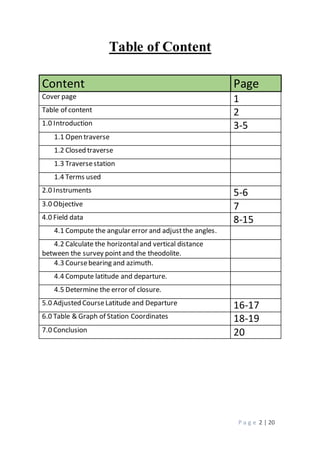
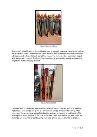
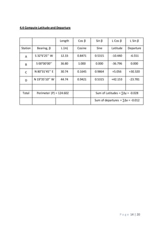
4.5 Determine The Error of Closure
Accuracy = 1 : (P/Ec)
Ec = [(sum of latitude)² + (sumof departure)²]^½
= [(-0.028) ²+(-0.012) ²]^ ½
= 0.0305 m
Therefore, the accuracy is = 1 : ( 124.602/0.0305)
= 1 : 4085.3115
= 1 : 4085
For average land surveying an accuracy of about 1 : 3000 is typical.
Hence, the accuracy of field is acceptable.
Error in departure ∑∆x = -0.012m
Error in latitude ∑∆y = -0.028m
Total Error = 0.030m](https://image.slidesharecdn.com/sitesurveyreport2-171221190515/85/Site-survey-report-2-15-320.jpg)
![P a g e 16 | 20
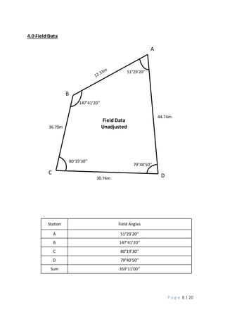
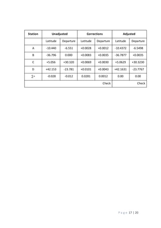
5.0 Adjusted Course Latitude and Departure
The Compass Pule
Correction = - [ΣΔy] / P x L or - [ΣΔx] / P x L
Where,
∑∆y and ∑∆x = the error in latitude or in departure
P = the total length or perimeter of the traverse
L = the length of a particular course
Latitude Correction
The correction to the latitude of course AB is
- (-0.028/124.602) × 12.325 = 0.0028
The correction to the latitude of course BC is
- (-0.028/124.602) x 36.796 = 0.0083
The correction to the latitude of course CD is
- (-0.028/124.602) x 30.738 = 0.0069
The correction to the latitude of course DA is
- (-0.028/124.602) x 44.743 = 0.0101
Departure Correction
The correction to the departure of course AB is
- (-0.012/124.602) × 12.325 = 0.0012
The correction to the departure of course BC is
- (-0.012/124.602) x 36.796 = 0.0035
The correction to the departure of course CD is
- (-0.012/124.602) x 30.738 = 0.0030
The correction to the departure of course DA is
- (-0.012/124.602) x 44.743 = 0.0043](https://image.slidesharecdn.com/sitesurveyreport2-171221190515/85/Site-survey-report-2-16-320.jpg)
![P a g e 19 | 20
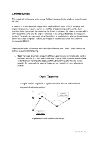
FIGURE The adjusted loop traverse plotted by coordinates.
Area = ½ x {[(EAxNB)+(EBxNC)+(ECxND)+(EDxNA)] -[(NAxEB)+(NBxEC)+(NCxED)+(NDxEA)]}
Area = ½ x {[(1000x989.563)+(993.450x952.775)+(993.454x957.838)+(1023.777)] –
[(1000x993.450)+(989.563x993.454)+(952.775x1023.777)+(957.838x1000)]}
= 819.932](https://image.slidesharecdn.com/sitesurveyreport2-171221190515/85/Site-survey-report-2-19-320.jpg)