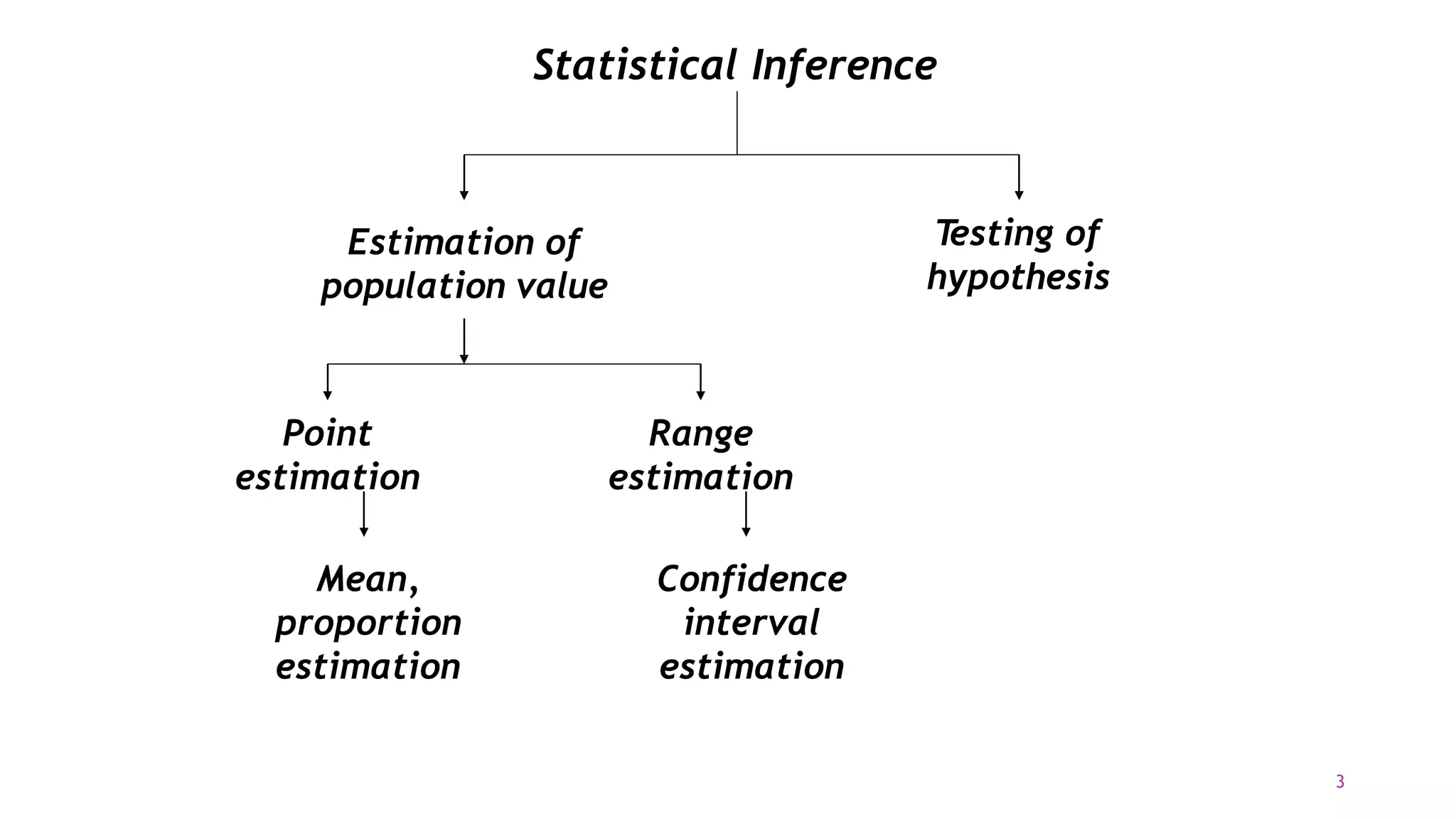
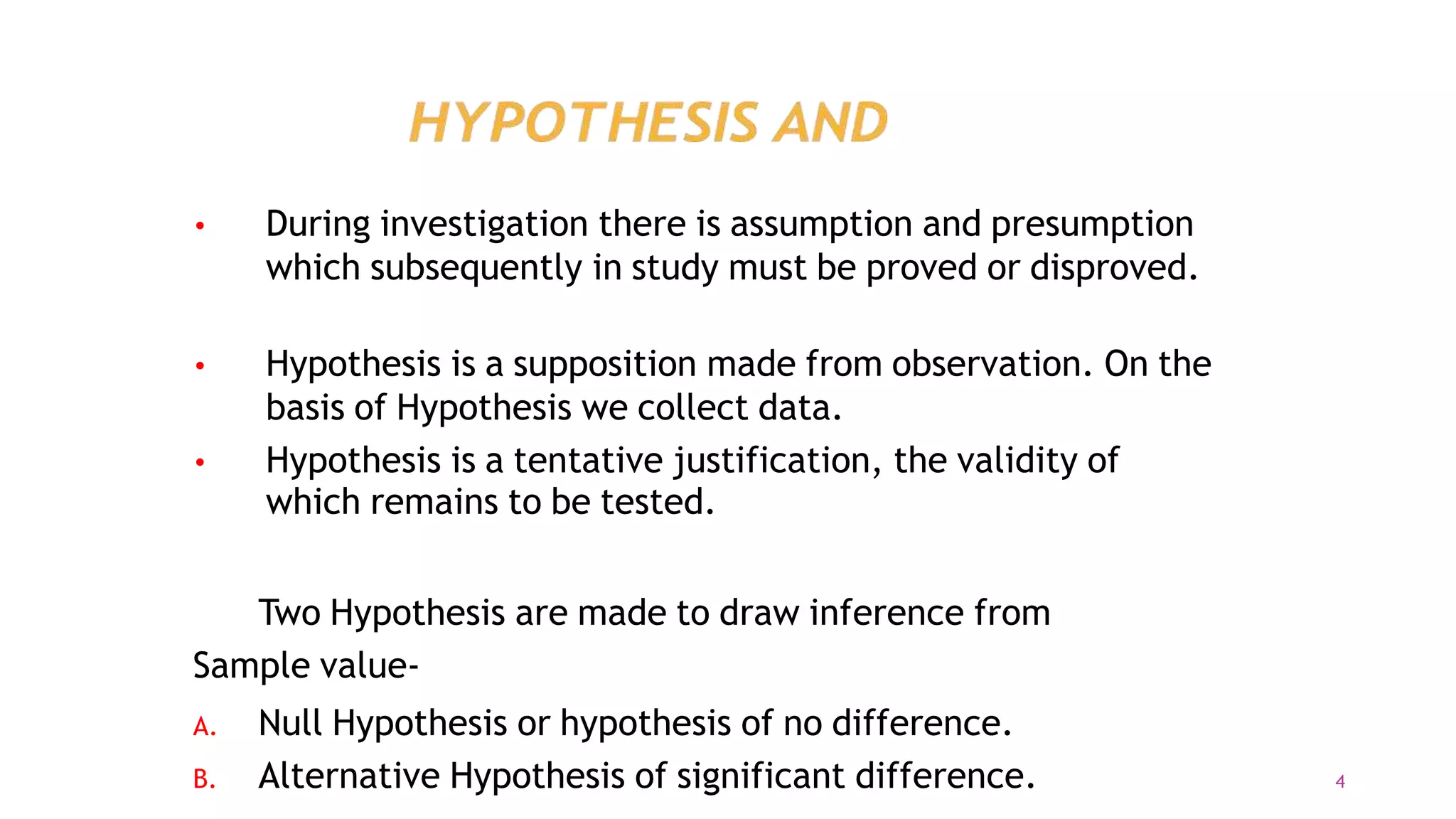
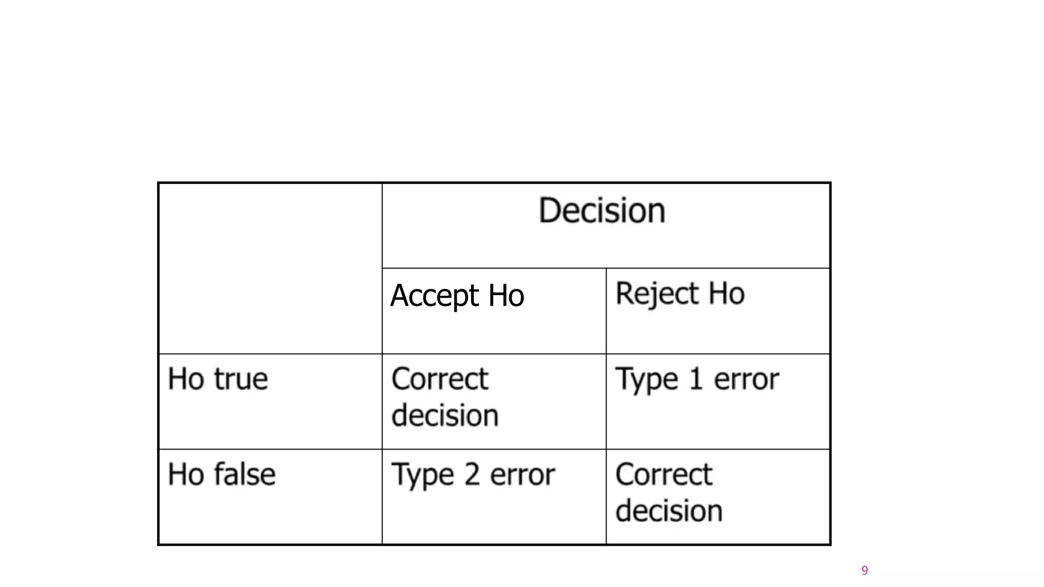
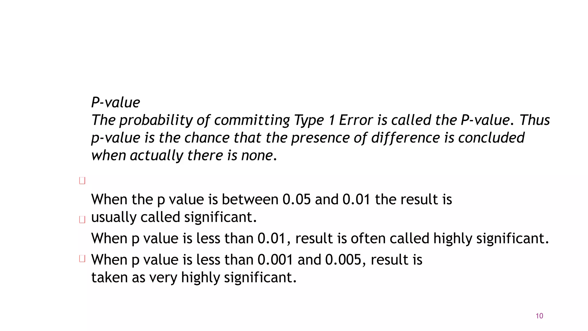
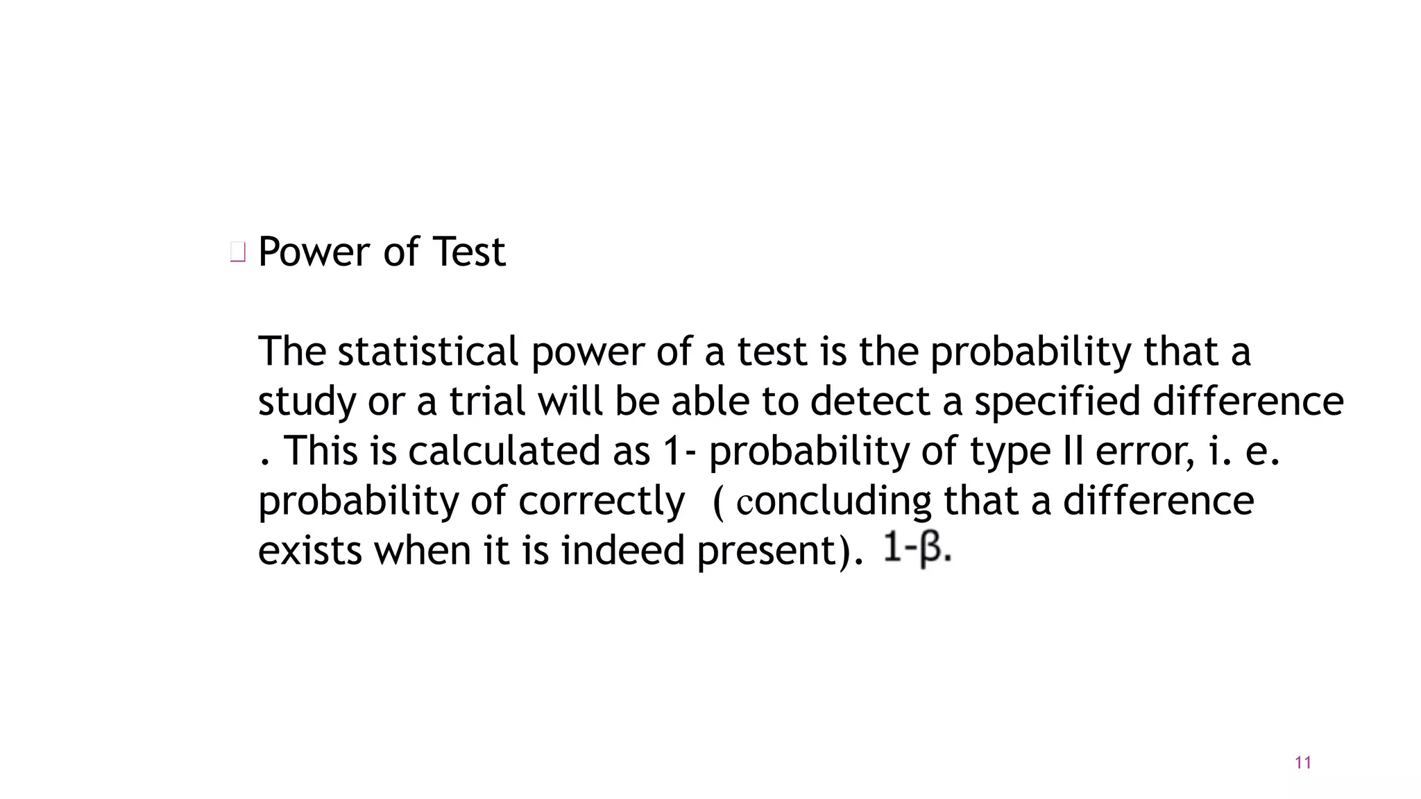
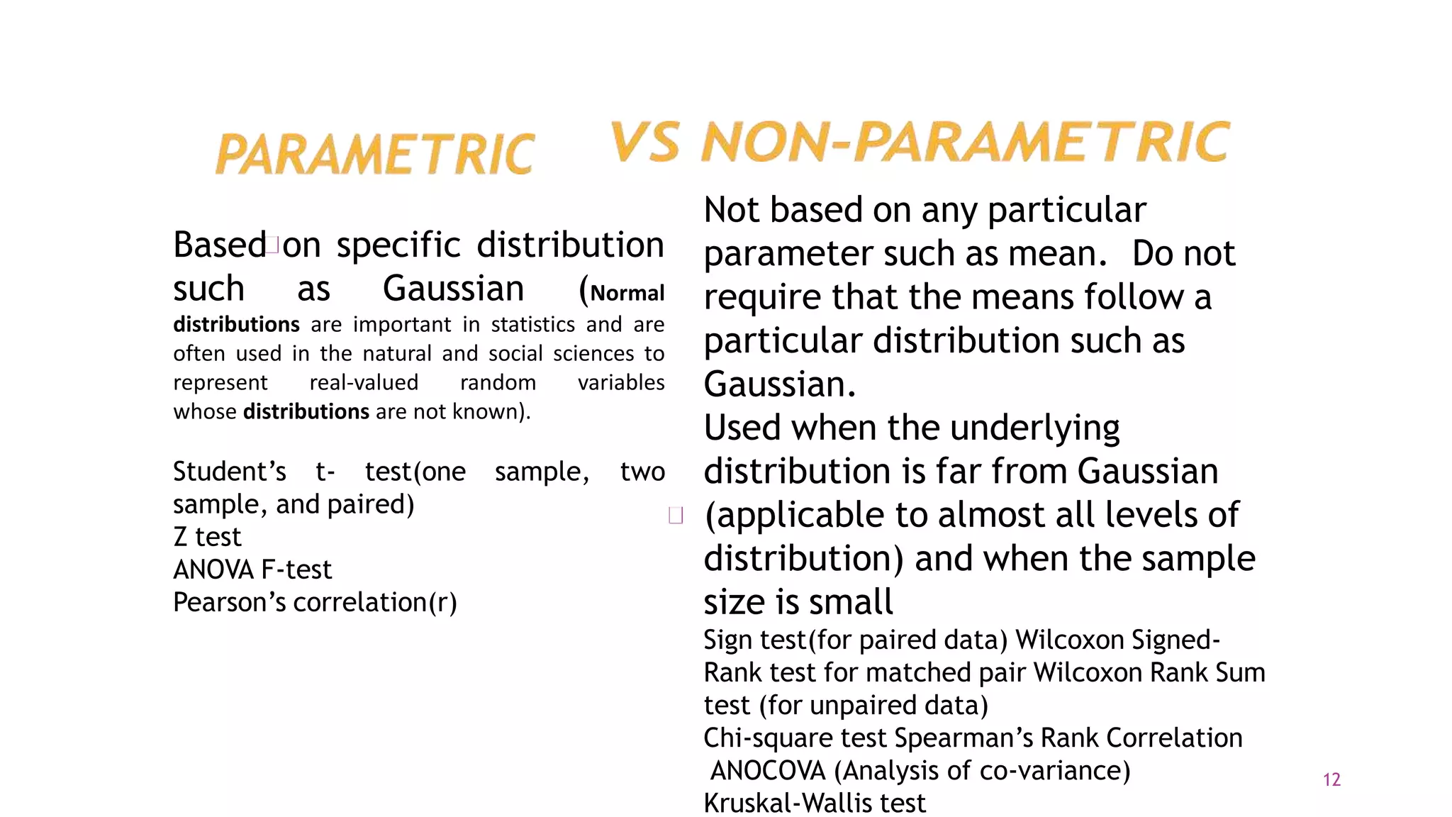
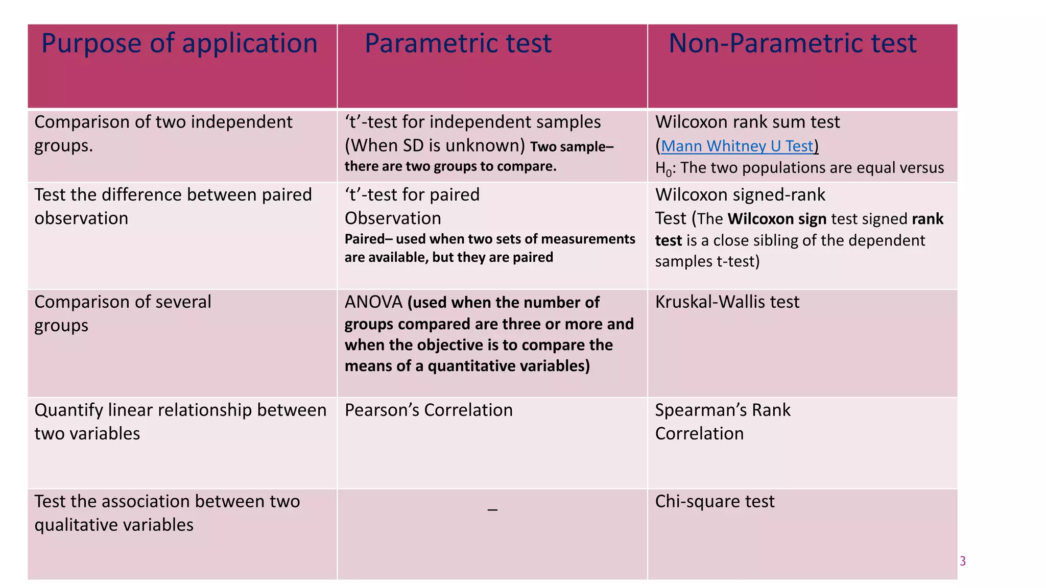
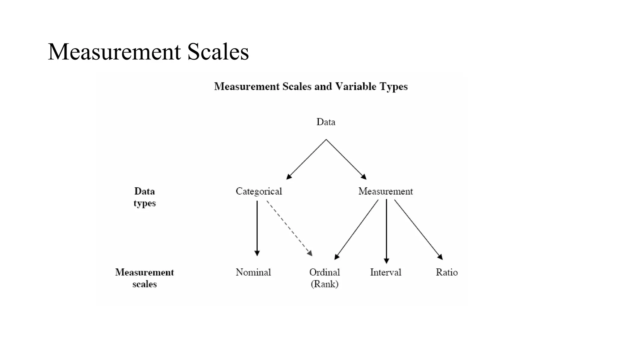
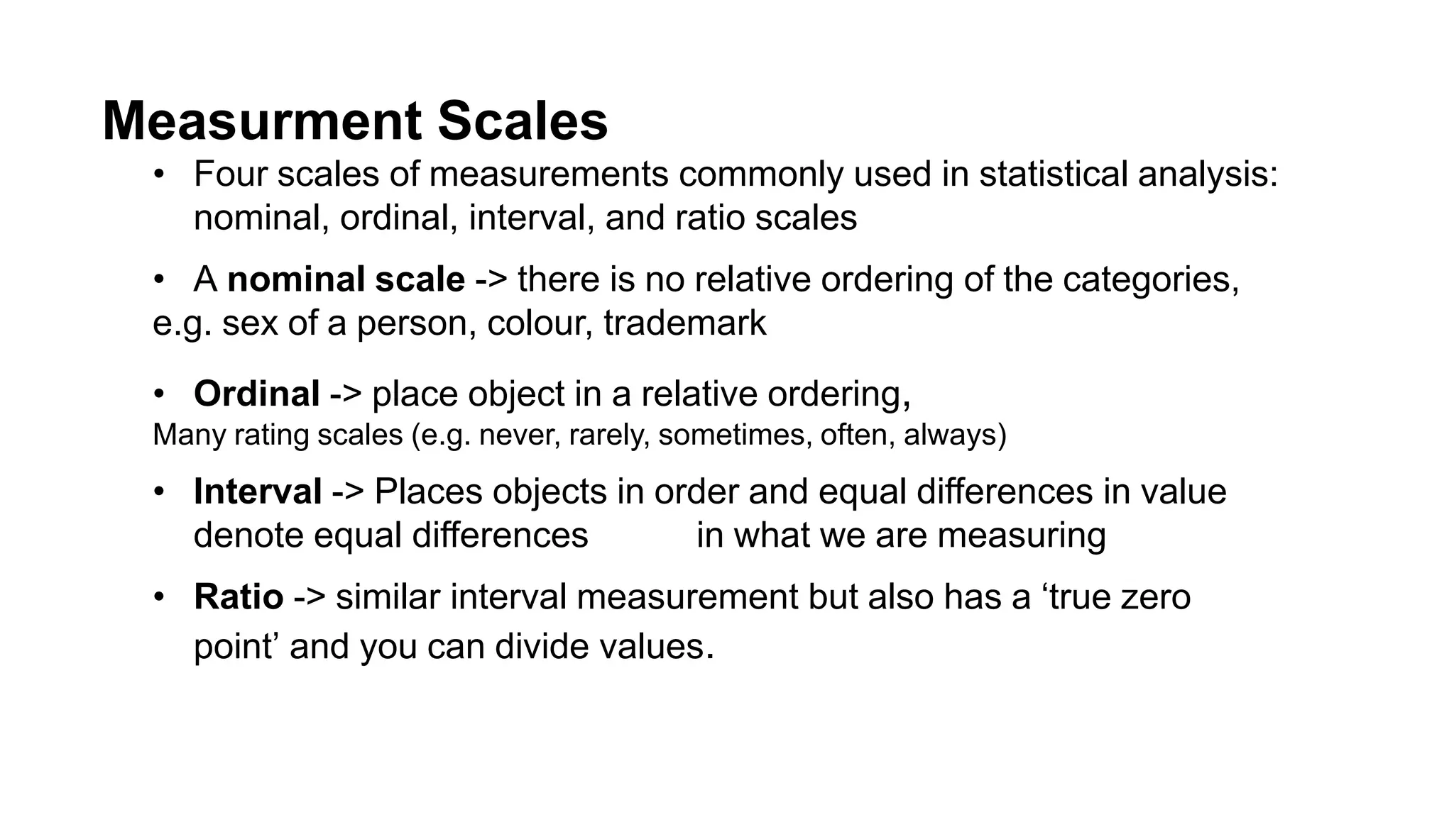
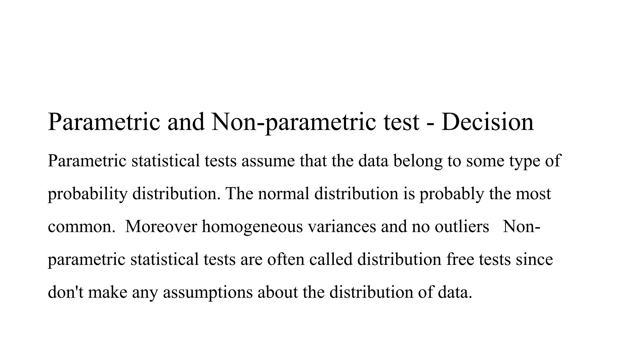
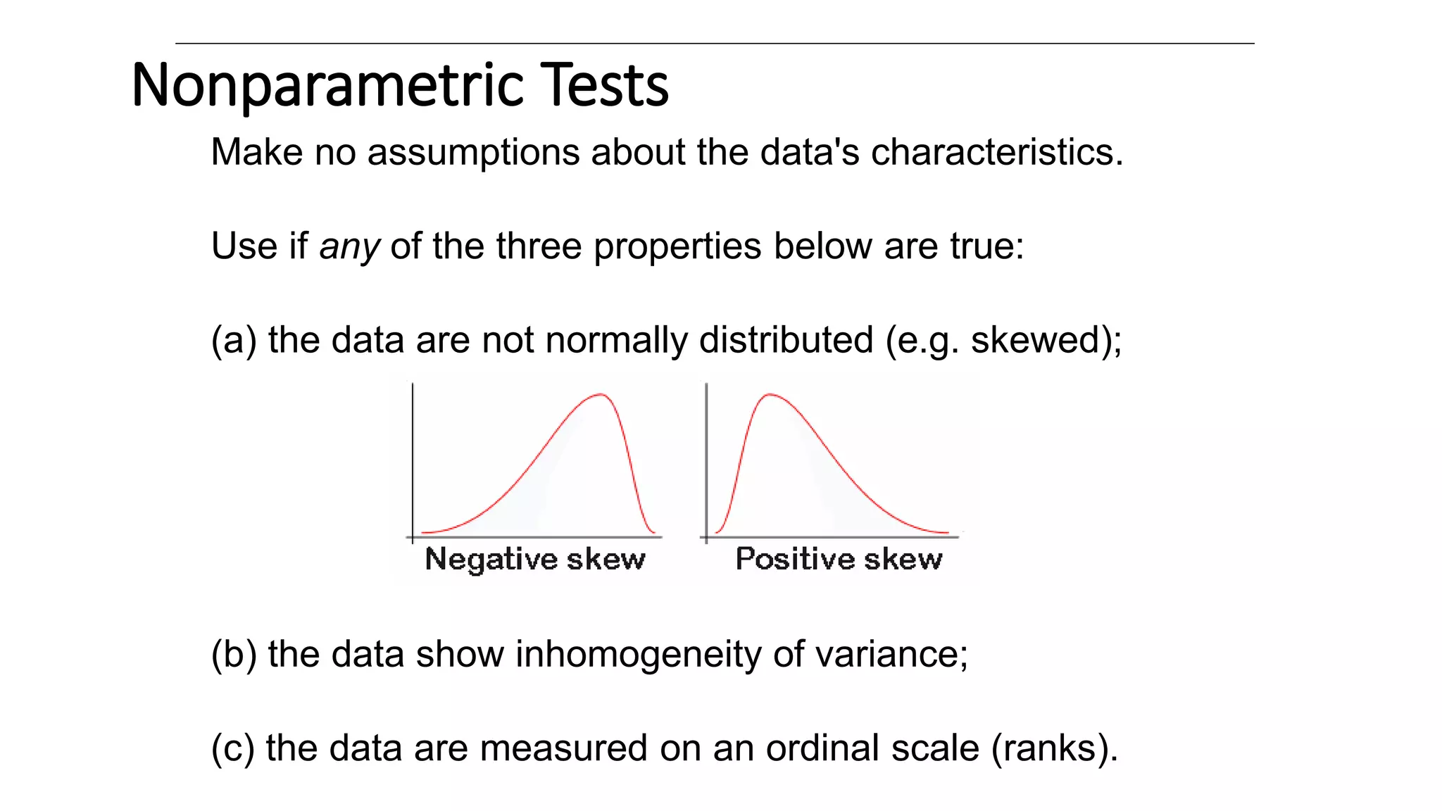
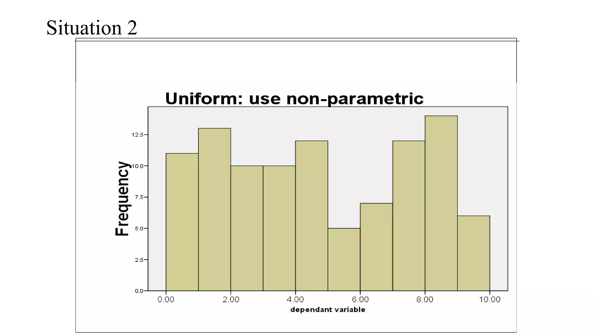
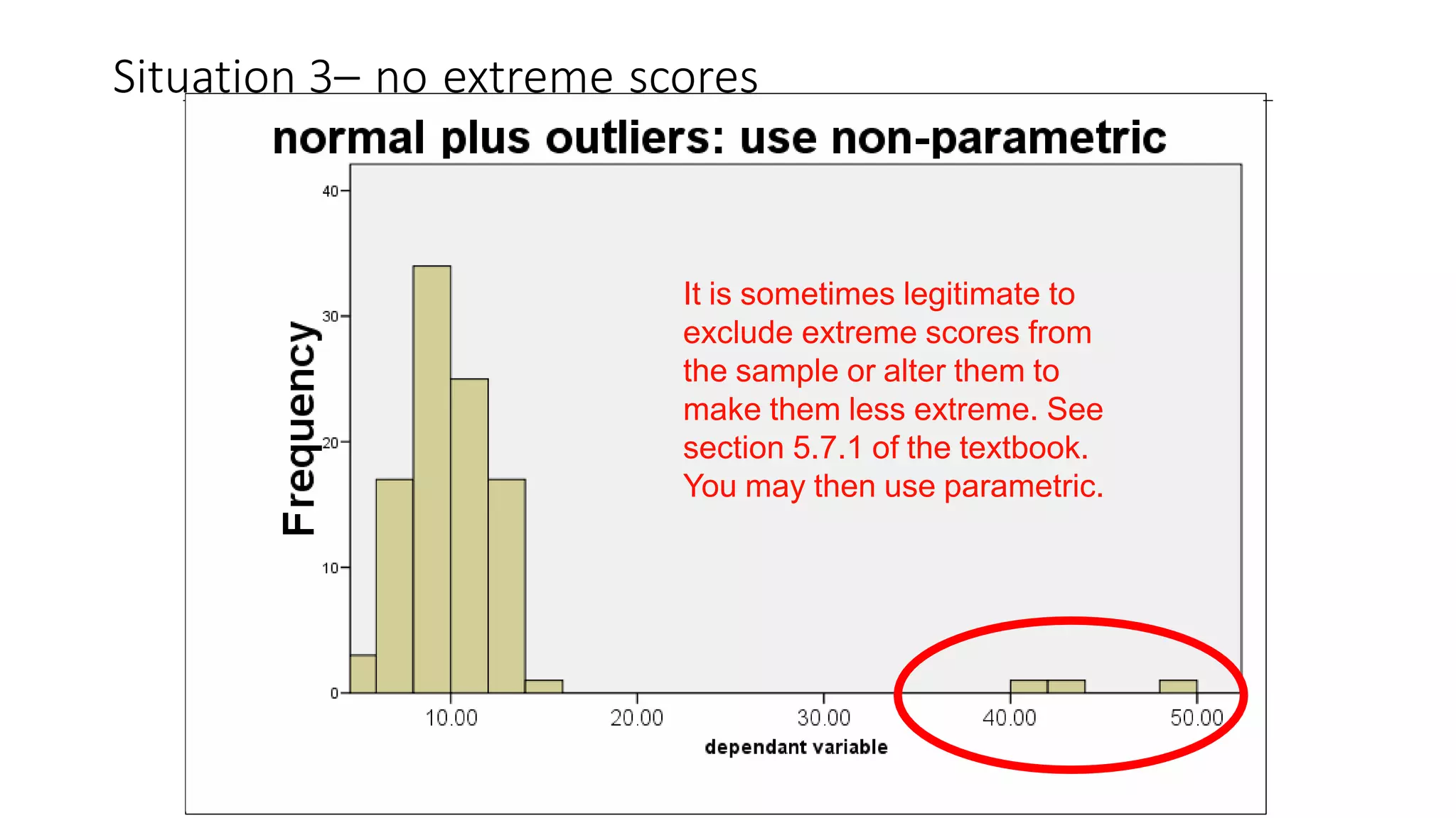
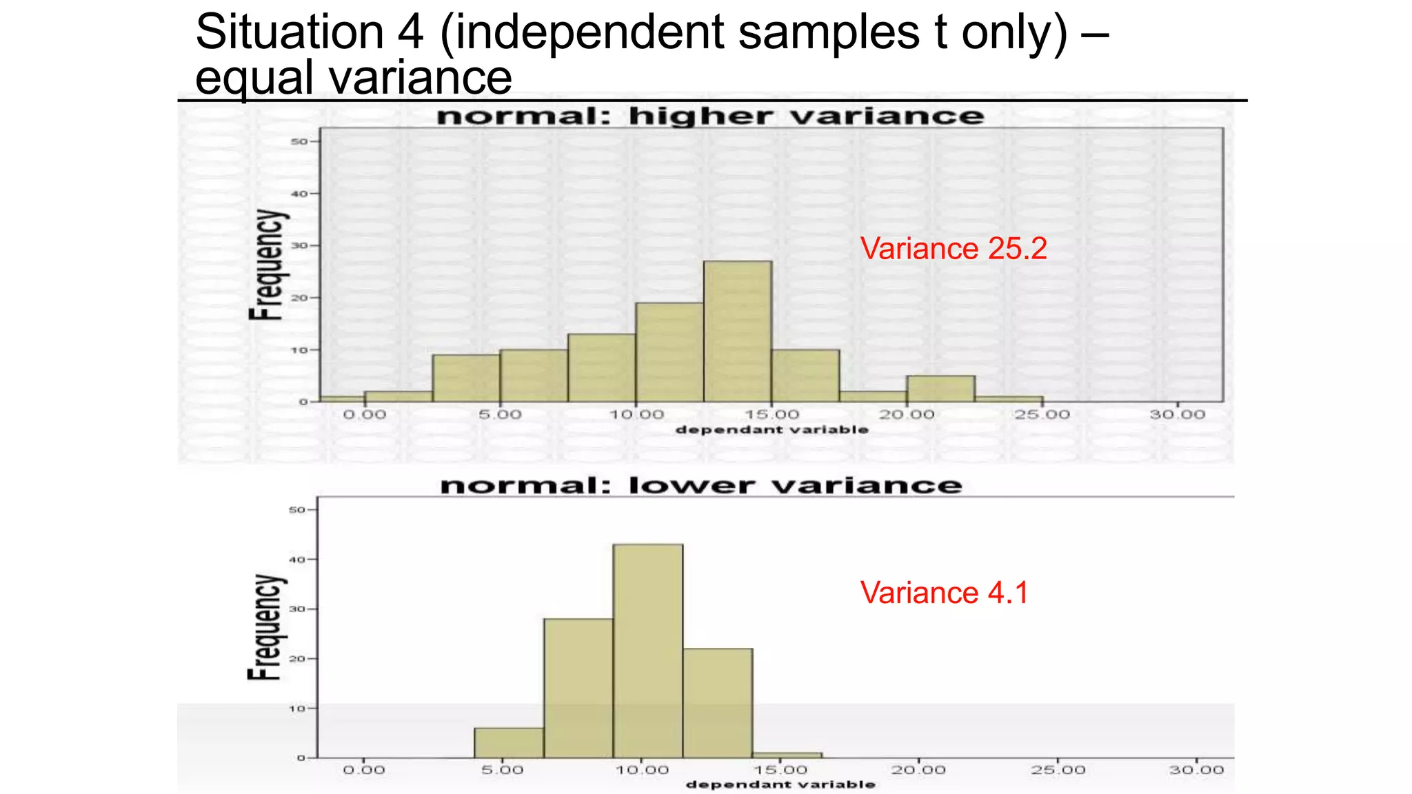
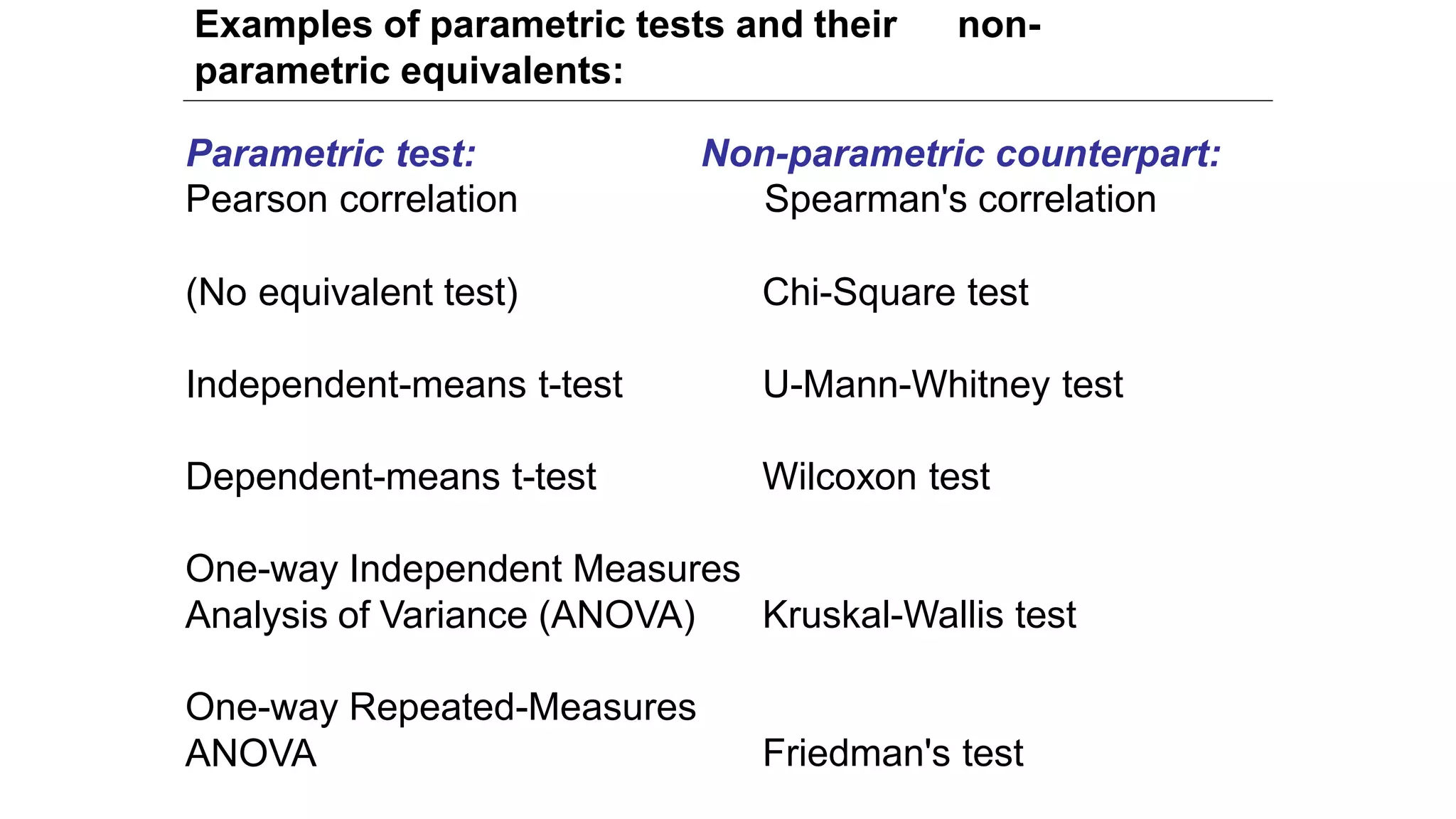
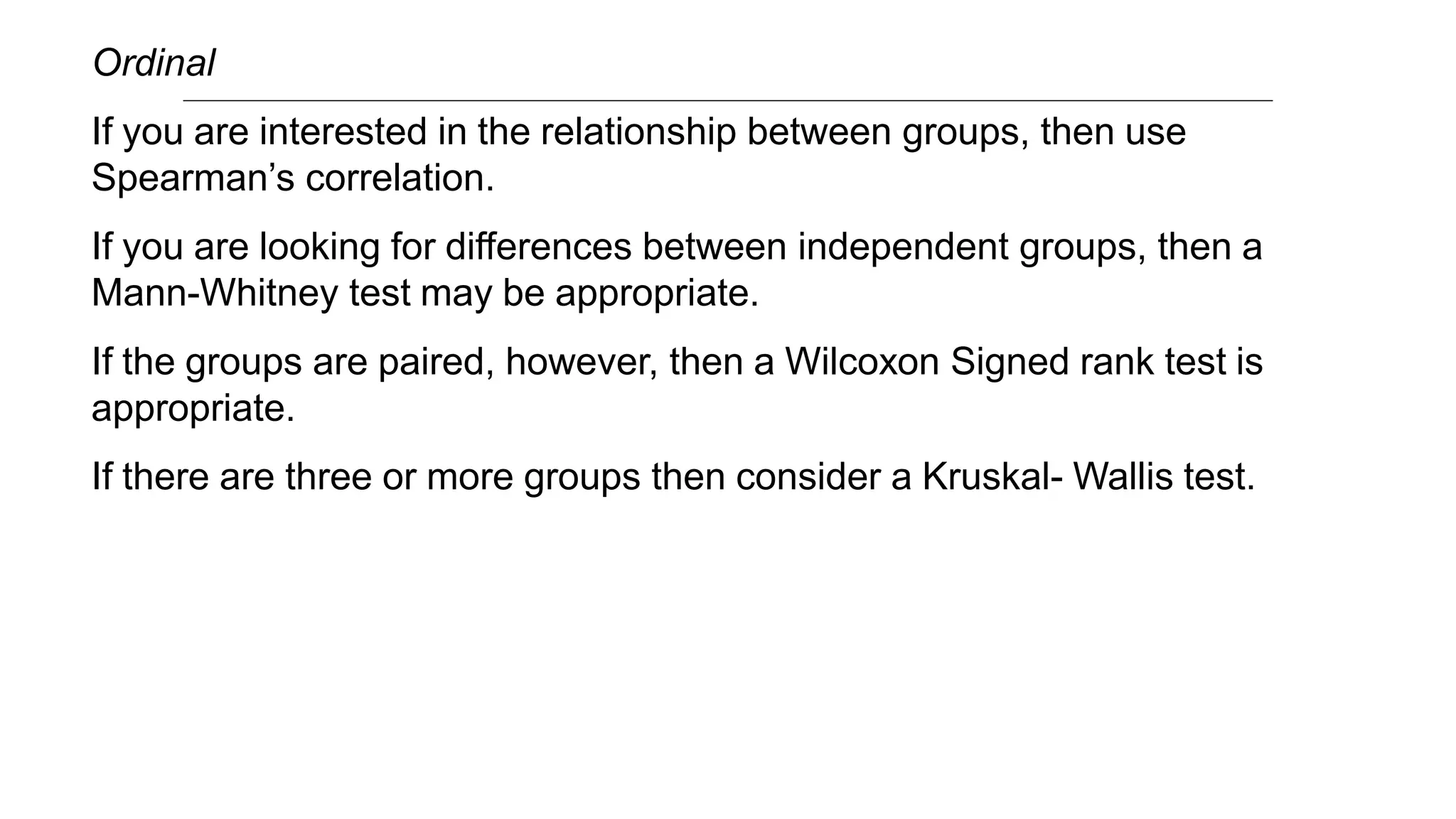
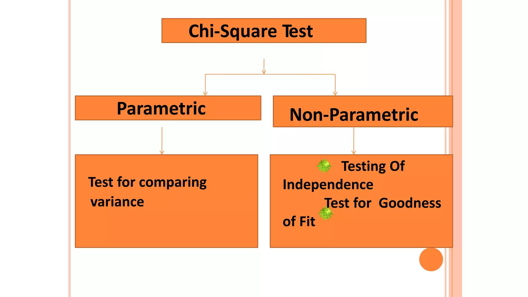
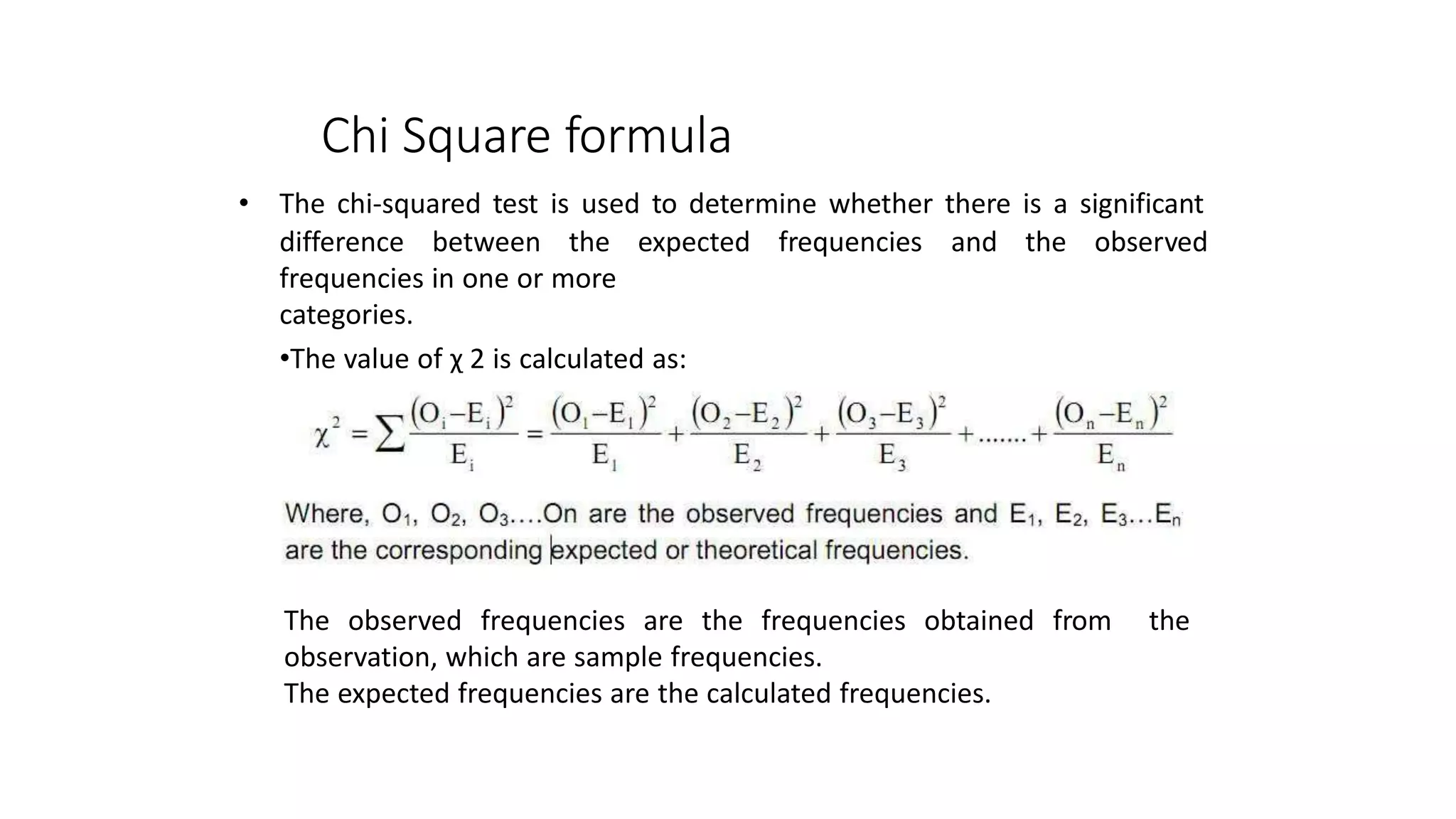
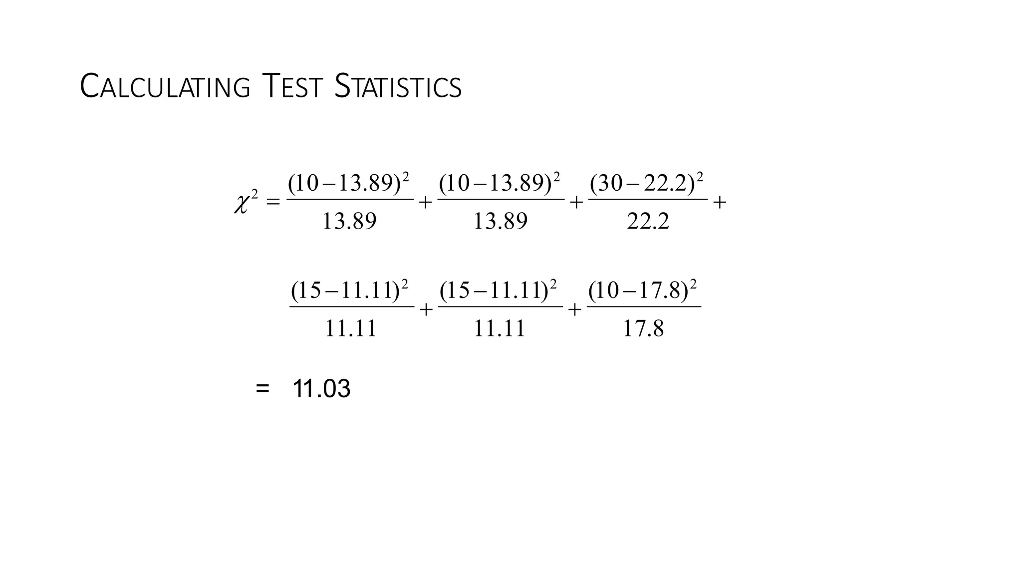
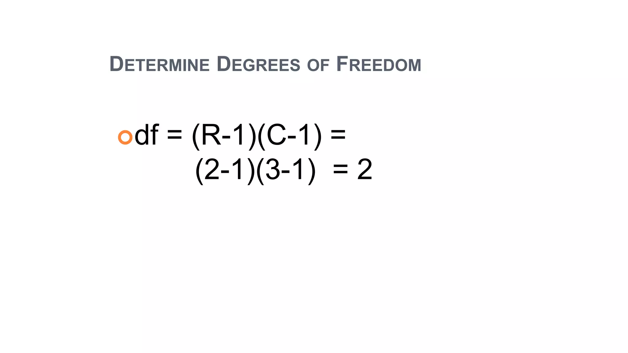
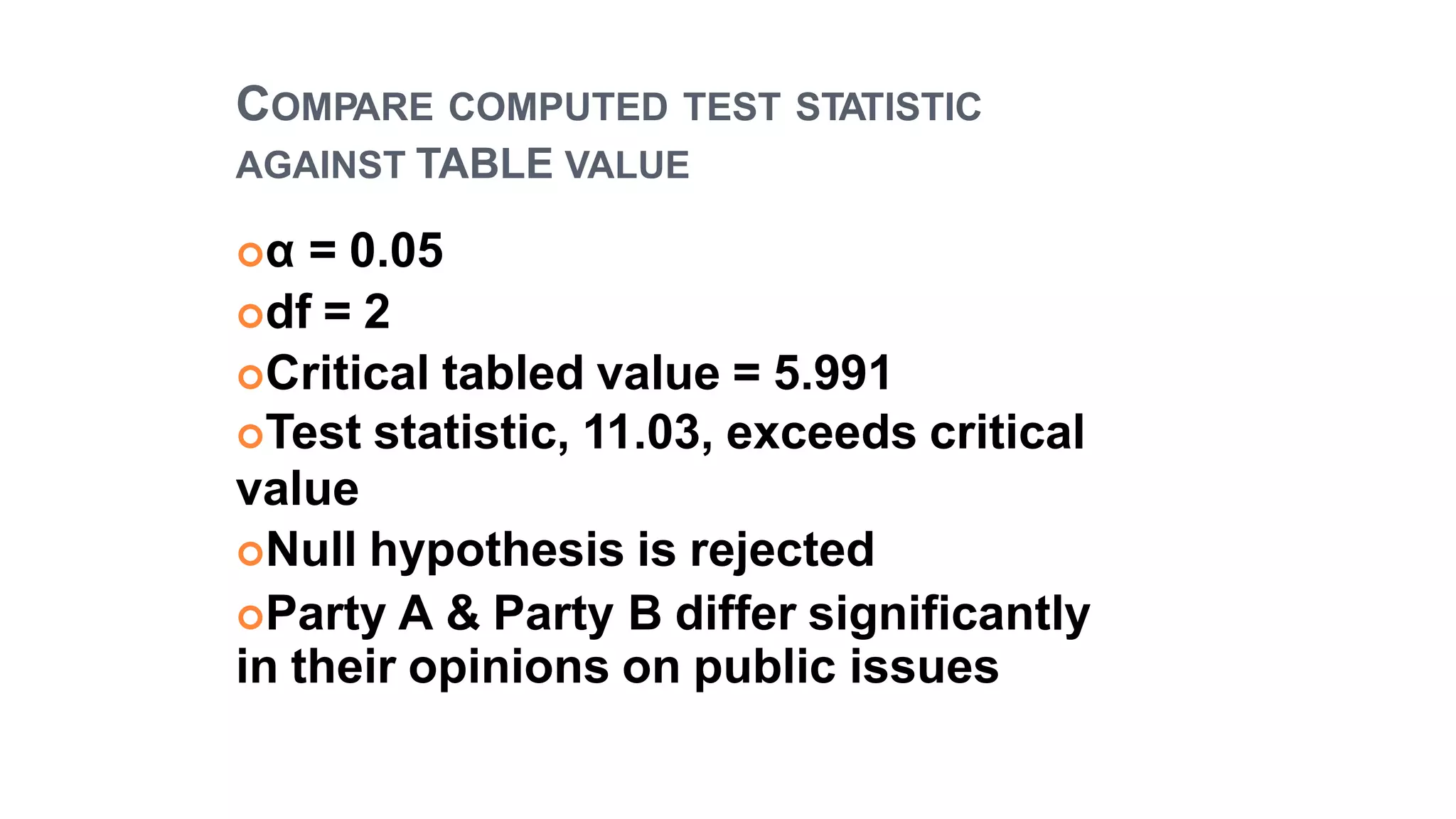
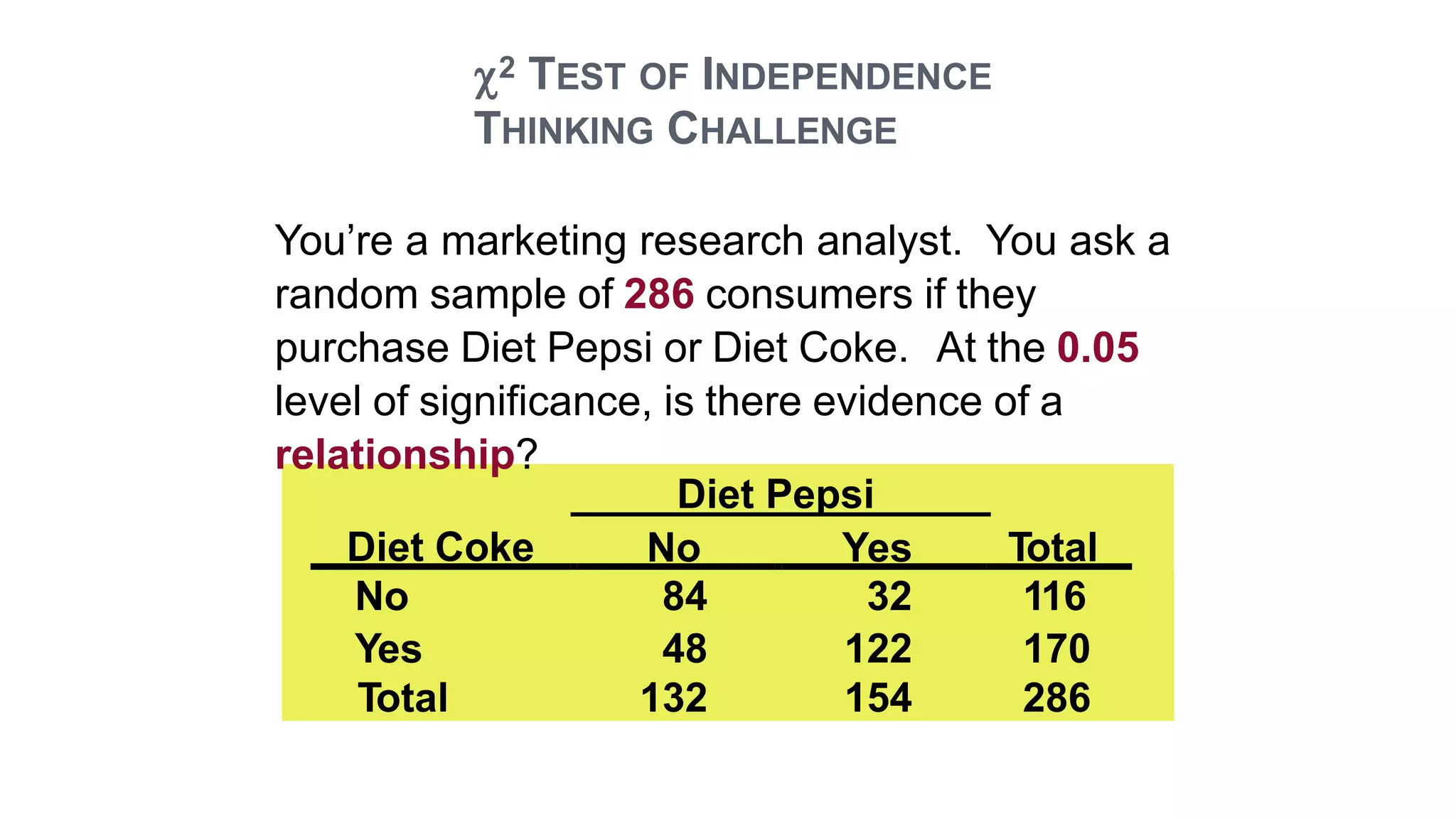
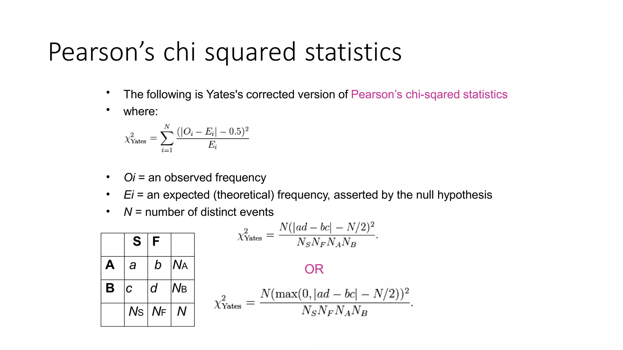
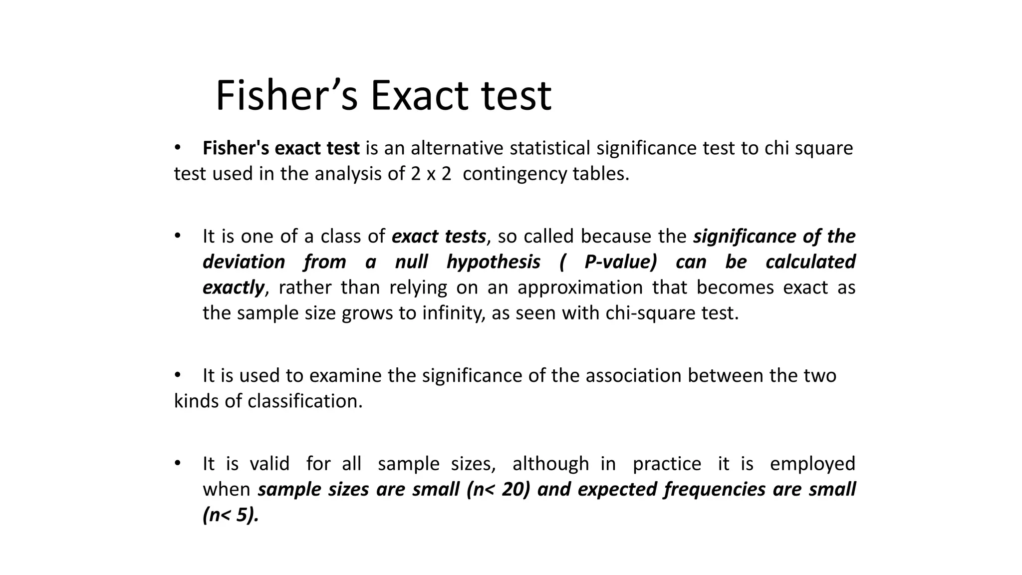
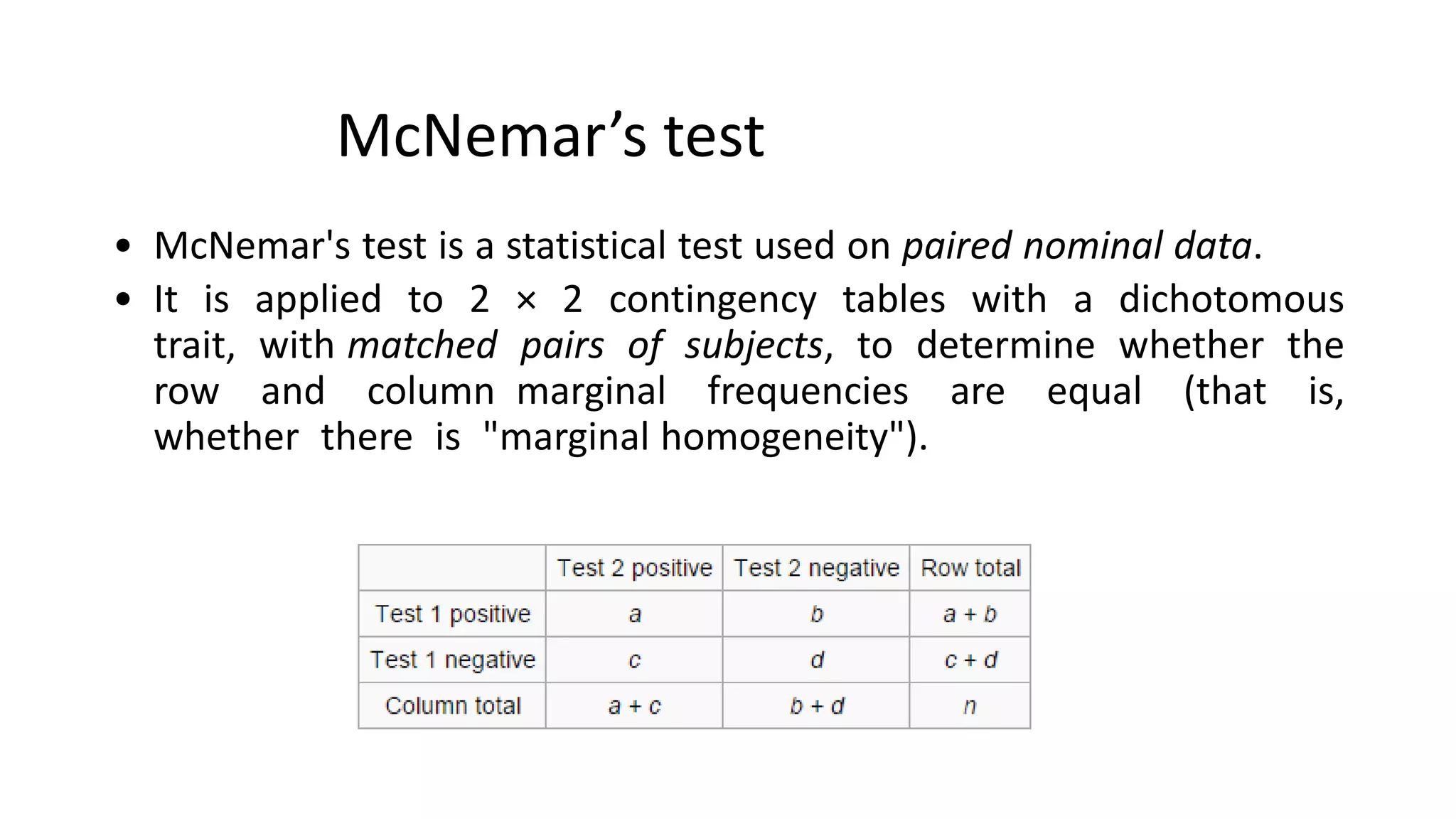
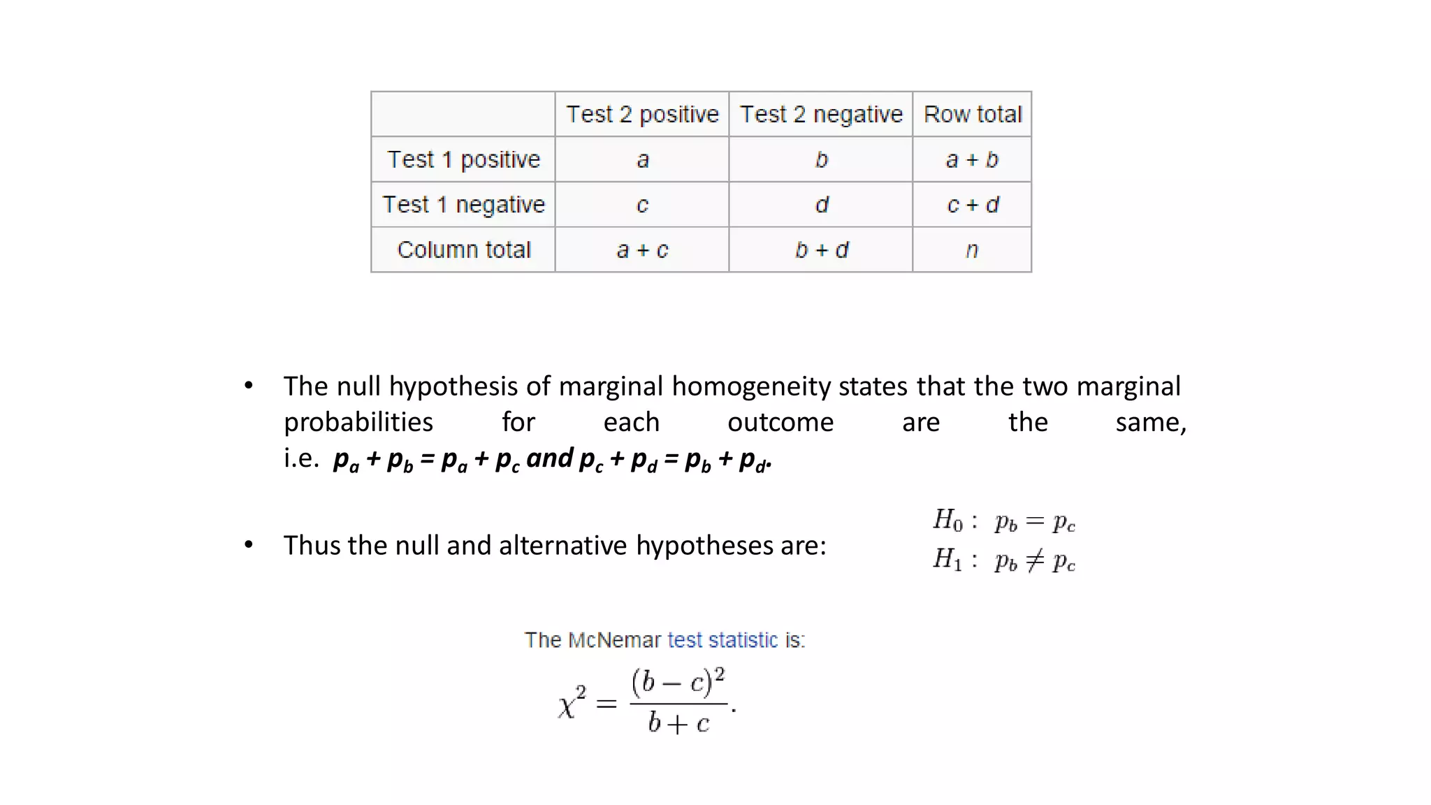
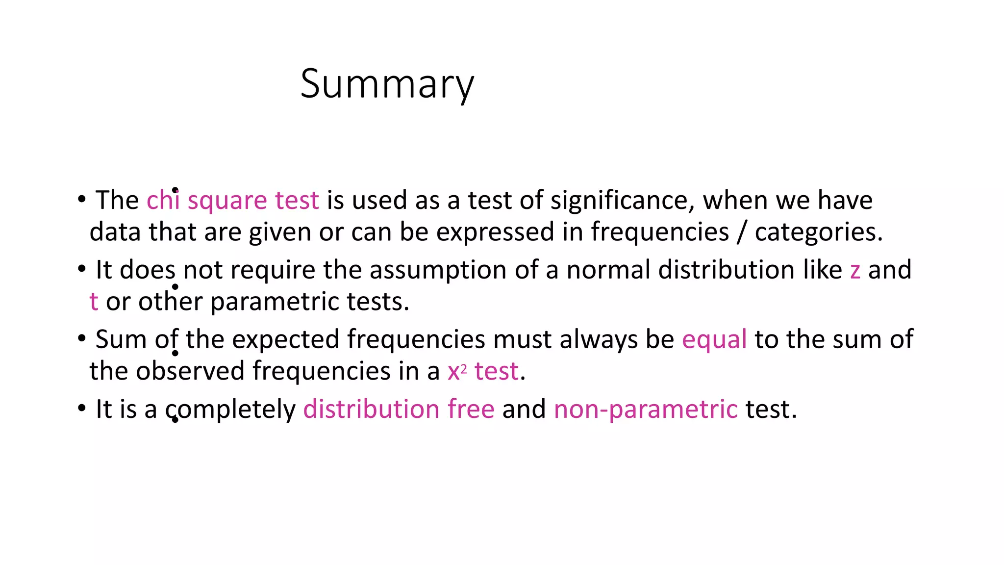
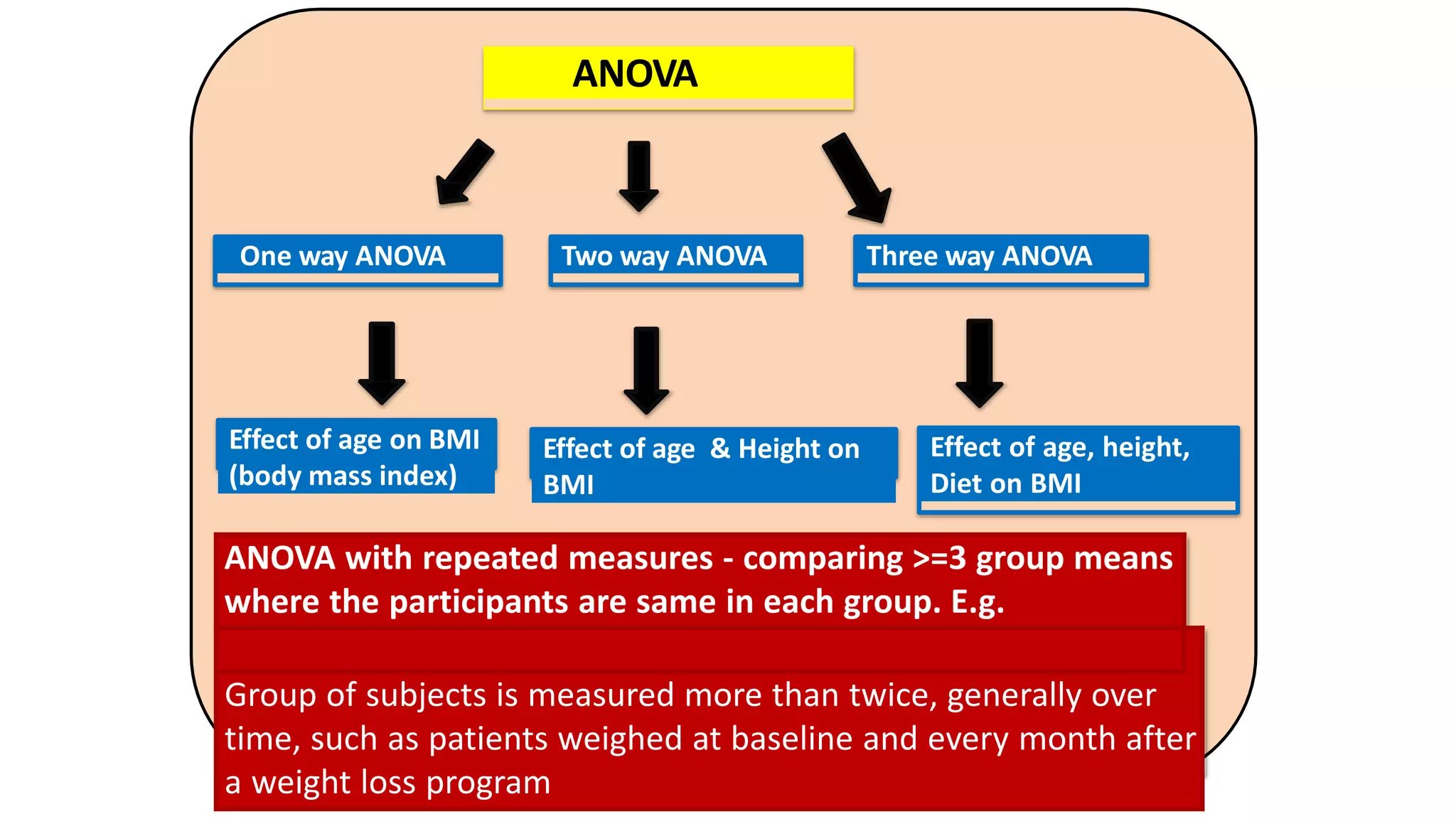
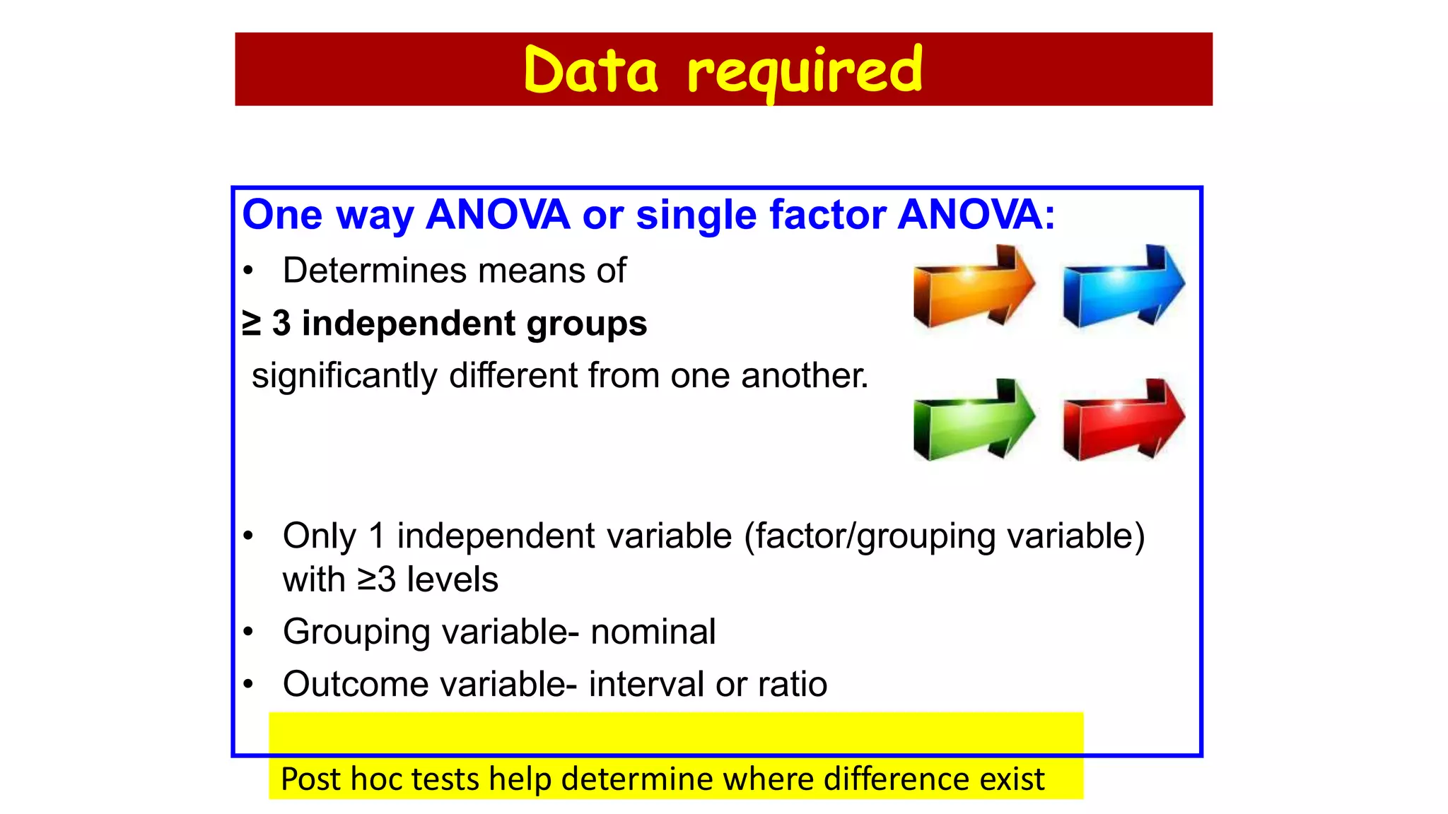
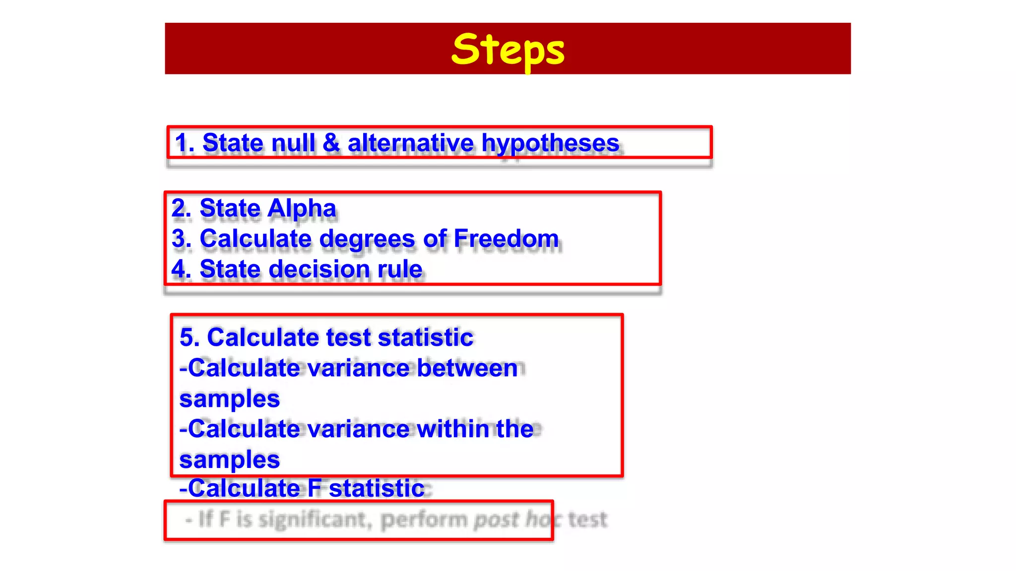
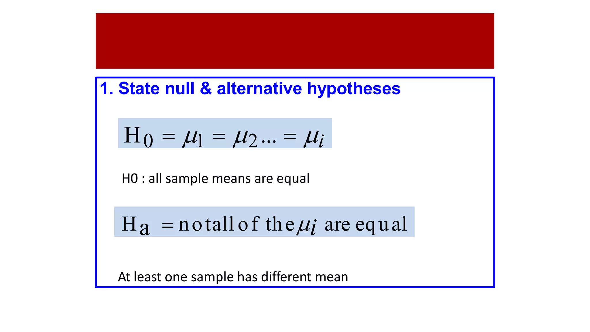
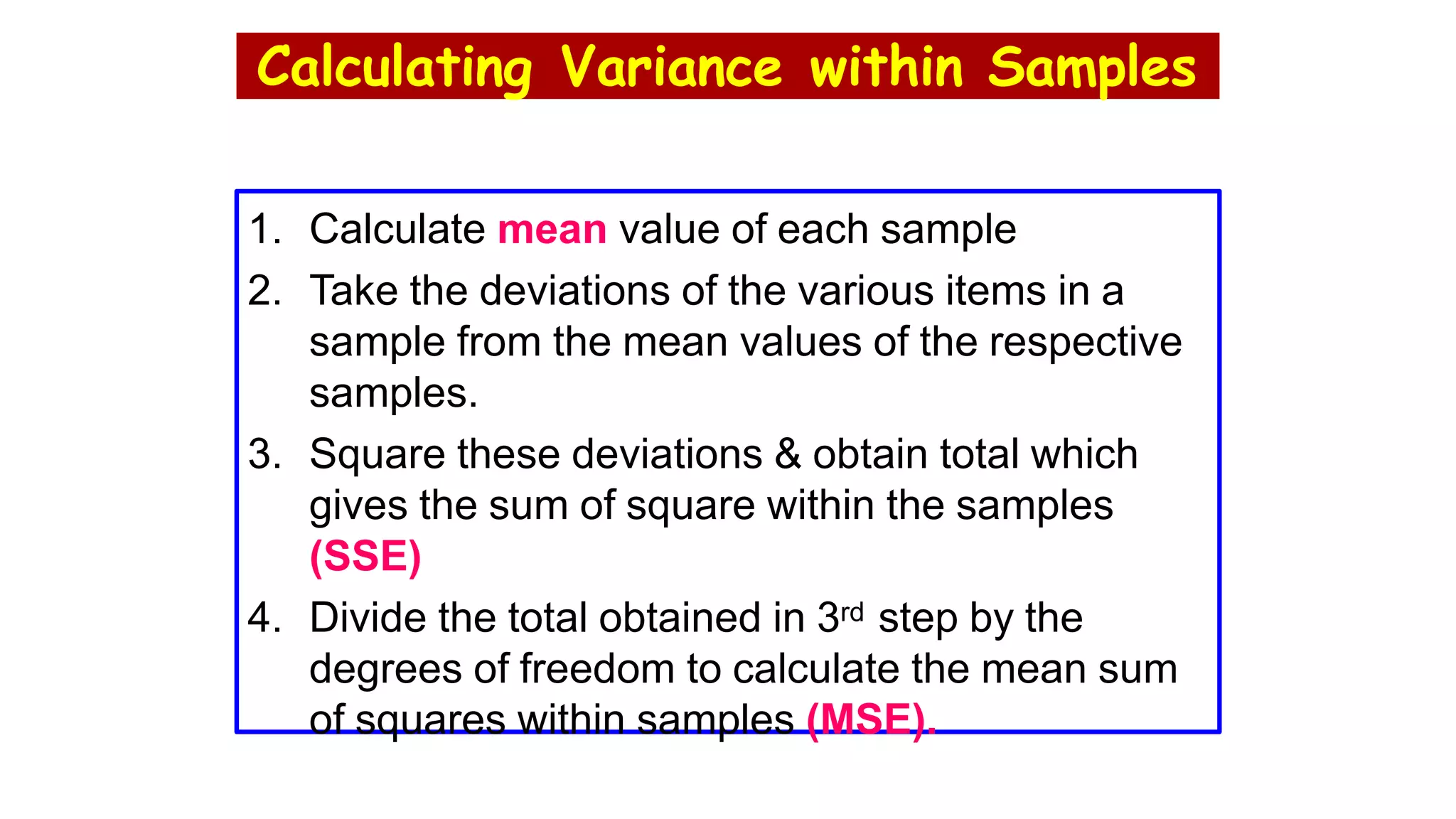
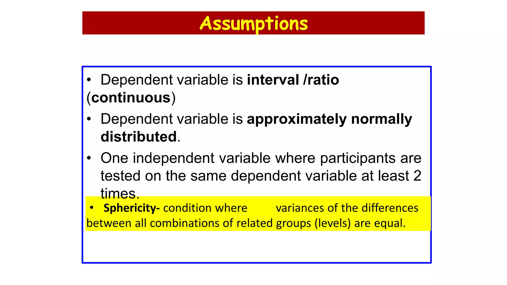
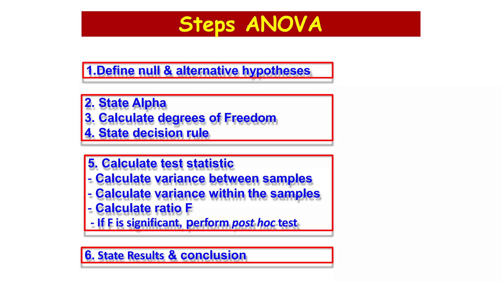
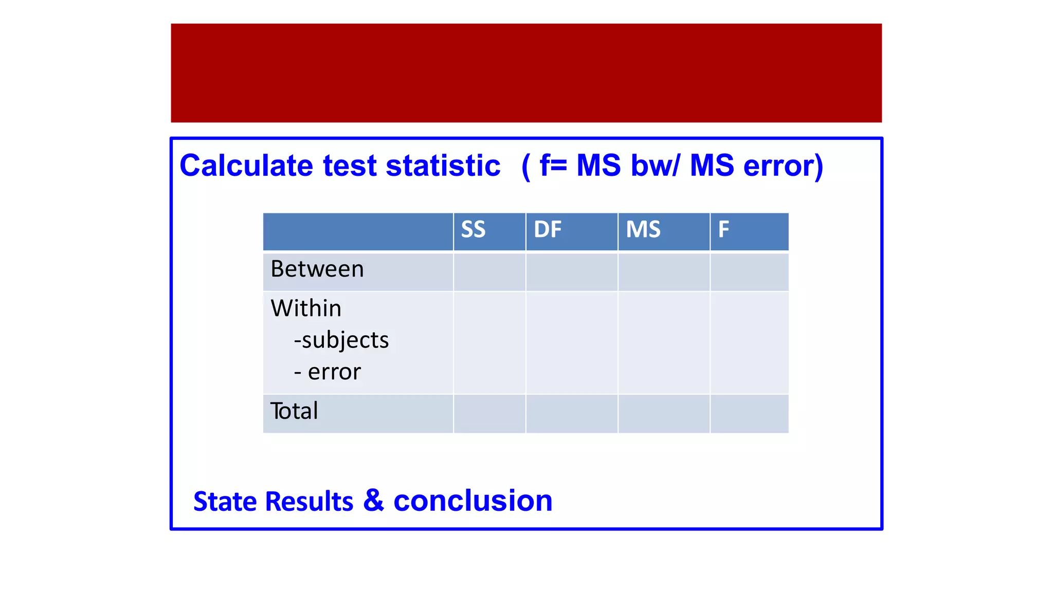
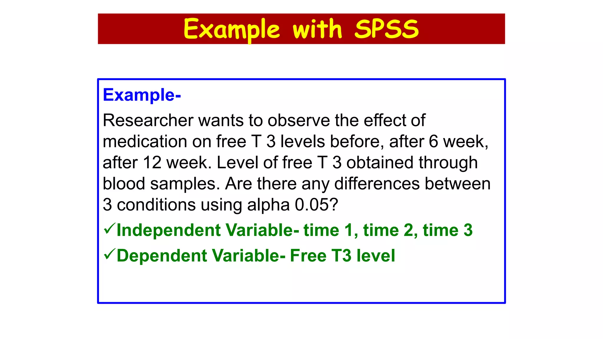
SlideShare a Scribd company logo
1 of 137
Non-Parametric Test
– Chi-Square Test
Dr. Sridhar L S
Faculty - SJCC
Statistical inference is the branch of statistics which is
concerned with using probability concept to deal with
certainly in decision making.
It refers to the process of selecting and using a sample to
draw inference about population from which sample is
drawn.
2
Statistical Inference
Estimation of
population value
Testing of
hypothesis
Point
estimation
Range
estimation
Mean,
proportion
estimation
Confidence
interval
estimation
3
•
4
During investigation there is assumption and presumption
which subsequently in study must be proved or disproved.
• Hypothesis is a supposition made from observation. On the
basis of Hypothesis we collect data.
Hypothesis is a tentative justification, the validity of
which remains to be tested.
•
Two Hypothesis are made to draw inference from
Sample value-
A. Null Hypothesis or hypothesis of no difference.
B. Alternative Hypothesis of significant difference.
The Null Hypothesis is symbolized as H0 and
Alternative Hypothesis is symbolized as H1 or HA.
In Hypothesis testing we proceed on the basis of
Null Hypothesis. We always keep Alternative
Hypothesis in mind.
The Null Hypothesis and the Alternative
Hypothesis are chosen before the sample is
drawn.
5
A Null Hypothesis or Hypothesis of no difference
(Ho) between statistic of a sample and parameter of
population or between statistic of two samples
nullifies the claim that the experimental result is
different from or better than the one observed
already. In other words, Null Hypothesis states that
the observed difference is entirely due to sampling
error, that is - it has occurred purely by chance.
6
Accept H0
Reject H0 Reject H0
Zcrit Zcrit
Setting a criterion
0
H
Null Hypothesis
7
When a Null Hypothesis is tested, there may be four
possible outcomes:
i. The Null Hypothesis is true but our test rejects it.
ii. The Null Hypothesis is false but our test accepts it.
iii.The Null Hypothesis is true and our test accepts it.
iv.The Null Hypothesis is false but our test rejects it.
Type 1 Error – rejecting Null Hypothesis when Null
Hypothesis is true.
Type 2 Error – accepting Null Hypothesis when Null
Hypothesis is false.
8
Accept Ho
9
P-value
The probability of committing Type 1 Error is called the P-value. Thus
p-value is the chance that the presence of difference is concluded
when actually there is none.
When the p value is between 0.05 and 0.01 the result is
usually called significant.
When p value is less than 0.01, result is often called highly significant.
When p value is less than 0.001 and 0.005, result is
taken as very highly significant.
10
Power of Test
The statistical power of a test is the probability that a
study or a trial will be able to detect a specified difference
. This is calculated as 1- probability of type II error, i. e.
probability of correctly ( concluding that a difference
exists when it is indeed present).
11
Based on specific distribution
such as Gaussian (Normal
distributions are important in statistics and are
often used in the natural and social sciences to
represent real-valued random variables
whose distributions are not known).
Student’s t- test(one sample, two
sample, and paired)
Z test
ANOVA F-test
Pearson’s correlation(r)
Not based on any particular
parameter such as mean. Do not
require that the means follow a
particular distribution such as
Gaussian.
Used when the underlying
distribution is far from Gaussian
(applicable to almost all levels of
distribution) and when the sample
size is small
Sign test(for paired data) Wilcoxon Signed-
Rank test for matched pair Wilcoxon Rank Sum
test (for unpaired data)
Chi-square test Spearman’s Rank Correlation
ANOCOVA (Analysis of co-variance)
Kruskal-Wallis test
12
13
Purpose of application Parametric test Non-Parametric test
Comparison of two independent
groups.
‘t’-test for independent samples
(When SD is unknown) Two sample–
there are two groups to compare.
Wilcoxon rank sum test
(Mann Whitney U Test)
H0: The two populations are equal versus
Test the difference between paired
observation
‘t’-test for paired
Observation
Paired– used when two sets of measurements
are available, but they are paired
Wilcoxon signed-rank
Test (The Wilcoxon sign test signed rank
test is a close sibling of the dependent
samples t-test)
Comparison of several
groups
ANOVA (used when the number of
groups compared are three or more and
when the objective is to compare the
means of a quantitative variables)
Kruskal-Wallis test
Quantify linear relationship between
two variables
Pearson’s Correlation Spearman’s Rank
Correlation
Test the association between two
qualitative variables
_ Chi-square test
Measurement Scales
Measurment Scales
• Four scales of measurements commonly used in statistical analysis:
nominal, ordinal, interval, and ratio scales
• A nominal scale -> there is no relative ordering of the categories,
e.g. sex of a person, colour, trademark
• Ordinal -> place object in a relative ordering,
Many rating scales (e.g. never, rarely, sometimes, often, always)
• Interval -> Places objects in order and equal differences in value
denote equal differences in what we are measuring
• Ratio -> similar interval measurement but also has a ‘true zero
point’ and you can divide values.
Parametric and Non-parametric test - Decision
Parametric statistical tests assume that the data belong to some type of
probability distribution. The normal distribution is probably the most
common. Moreover homogeneous variances and no outliers Non-
parametric statistical tests are often called distribution free tests since
don't make any assumptions about the distribution of data.
Nonparametric Tests
Make no assumptions about the data's characteristics.
Use if any of the three properties below are true:
(a) the data are not normally distributed (e.g. skewed);
(b) the data show inhomogeneity of variance;
(c) the data are measured on an ordinal scale (ranks).
This can be checked by inspecting a histogram with small samples the
histogram is unlikely to ever be exactly bell shaped
This assumption is only broken if there are large and obvious
departures from normality
Assumption 1 - normality
Situation 1
In severe skew the most
extreme histogram interval
usually has the highest
frequency
Situation 2
Situation 3– no extreme scores
It is sometimes legitimate to
exclude extreme scores from
the sample or alter them to
make them less extreme. See
section 5.7.1 of the textbook.
You may then use parametric.
Situation 4 (independent samples t only) –
equal variance
Variance 4.1
Variance 25.2
Parametric test:
Pearson correlation
Non-parametric counterpart:
Spearman's correlation
(No equivalent test) Chi-Square test
Independent-means t-test U-Mann-Whitney test
Dependent-means t-test Wilcoxon test
One-way Independent Measures
Analysis of Variance (ANOVA) Kruskal-Wallis test
One-way Repeated-Measures
ANOVA Friedman's test
Examples of parametric tests and their non-
parametric equivalents:
WHICH TEST SHOULD I USE?
The type of data that you collect will be important in your final choice of
test:
Nominal
Consider a chi-squared test if you are interested in differences in
frequency counts using nominal data, for example comparing whether
month of birth affects the sport that someone participates in.
Ordinal
If you are interested in the relationship between groups, then use
Spearman’s correlation.
If you are looking for differences between independent groups, then a
Mann-Whitney test may be appropriate.
If the groups are paired, however, then a Wilcoxon Signed rank test is
appropriate.
If there are three or more groups then consider a Kruskal- Wallis test.
Chi-Square Test
 Karl Pearson introduced a test to distinguish whether
an observed set of frequencies differs from a specified
frequency distribution
 The chi-square test uses frequency data to generate a
statistic
A chi-square test is a statistical test commonly used for
testing independence and goodness of fit. Testing
independence determines whether two or more observations
across two populations are dependent on each other (that is,
whether one variable helps to estimate the other).
Testing for goodness of fit determines if an observed
frequency distribution matches a theoretical frequency
distribution.
Chi-Square Test
Testing Of
Independence
Test for Goodness
of Fit
Test for comparing
variance
Non-ParametricParametric
Conditions for the application of 2 test
Observations recorded and collected on random
basis.
All items in the sample must beindependent.
No group should contain very few items, say less
than 5. (some statistician says less than 10) Total number
of items should be large, say at least 50.
The 2 distribution is not symmetrical and all the
values are positive. For each degrees of freedom
we have asymmetric curves.
1. Test for comparing variance
2 =
Chi- Square Test as a Non-Parametric Test
Test of Goodness of Fit.
Test of Independence.




(O  E) 

E
2
 2




(O  E)

E
2
 2
Steps involved
Determine The Hypothesis:
Ho : The two variables are independent
Ha : The two variables are associated
Calculate Expected frequency
Calculate test statistic
  

(O  E) 


E
2
 2
Determine Degrees of Freedom
df = (R-1)(C-1)
Compare computed test statistic against a tabled/critical
value
The computed value of the Pearson chi- square statistic is
compared with the critical value to determine if the computed value
is improbable
The critical tabled values are based on sampling distributions of
the Pearson chi- square statistic.
If calculated 2 is greater than 2 table value,reject Ho
Contingency table
• A contingency table is a type of table in a matrix format that
displays
the frequency distribution of the variables.
• They provide a basic picture of the interrelation between two variables and
can help find interactions between them.
• The chi-square statistic compares the observed count in each table cell to
the count which would be expected under the assumption of no association
between the row and column classifications.
Degrees of freedom
• The number of independent pieces of information which are free to vary,
that
go into the estimate of a parameter is called the degrees of freedom.
• In general, the degrees of freedom of an estimate of a parameter is equal to
the number of independent scores that go into the estimate minus
the number of parameters used as intermediate steps in the estimation of
the parameter itself (i.e. the sample variance has N-1 degrees of freedom,
since it is computed from N random scores minus the only 1 parameter
estimated as intermediate step, which is the sample mean).
• The number of degrees of freedom for ͚Ŷ͛ observations is ͚Ŷ-k͛ and is usually
denoted by ͚ʆ ͛, where ͚k͛ is the number of independent linear constraints
imposed upon them. It is the only parameter of the chi-square distribution.
• The degrees of freedom for a chi squared contingency table can be
calculated as:
• The chi-squared test is used to determine whether there is a significant
difference between the expected
frequencies in one or more
categories.
•The value of χ 2 is calculated as:
frequencies and the observed
The observed frequencies are the frequencies obtained
observation, which are sample frequencies.
The expected frequencies are the calculated frequencies.
from the
Chi Square formula
Critical values of 2
As a Manager, you want to test
the perception of fairness of
three methods of performance
evaluation. Of 180 employees, 63
rated
Method 1 as fair, 45 rated
Method 2 as fair, 72 rated
Method 3 as fair. At the 0.05
level of significance, is there a
difference in perceptions?
EXAMPLE
SOLUTION
Observed
frequency
Expected
frequency
(O-E) (O-E)2 (O-E)2
E
63 60 3 9 0.15
45 60 -15 225 3.75
72 60 12 144 2.4
6.3
Test Statistic:
2 = 6.3
Decision:
Reject H0 at sign. level 0.05
Conclusion:
At least 1 proportion is different
H0:
0
H1: At least 1 is
different
  = 0.05
 n1 = 63 n2 = n3 =
 Critical Value(s):
2
Reject H0
p1 = p2 = p3 = 1/3
45 72
5.991
 = 0.05
EXAMPLE
 Suppose a researcher is interested in voting
preferences on Public issues.
 A questionnaire was developed and sent to a
random sample of 90 voters.
 The researcher also collects information about
the political party membership of the sample of
90 respondents.
BIVARIATE FREQUENCY TABLE OR
CONTINGENCY TABLE
Favor Neutral Oppose f row
Party A 10 10 30 50
Party B 15 15 10 40
f column 25 25 40 n = 90
BIVARIATE FREQUENCY TABLE OR
CONTINGENCY TABLE
Favor Neutral Oppose f row
Democrat 10 10 30 50
Republican 15 15 10 40
f column 25 25 40 n = 90
2
2
BIVARIATE FREQUENCY TABLE OR
CONTINGENCY TABLE
Rowfrequency
Favor Neutral Oppose f row
Party A 10 10 30 50
Party B 15 15 10 40
f column 25 25 40 n = 90
BIVARIATE FREQUENCY TABLE OR
CONTINGENCY TABLE
Col
Favor Neutral Oppose f row
Party A 10 10 30 50
Party B 15 15 10 40
f column
umn frequency
25 25 40 n = 90
DETERMINE THE HYPOTHESIS
• Ho : There is no difference between A &
B in their opinion on Public issue.
• Ha : There is an association between
responses to public issue survey and
the party membership in the population.
CALCULATING TEST STATISTICS
Favor Neutral Oppose f row
Party A fo =10
fe =13.9
fo =10
fe =13.9
fo =30
fe=22.2
50
Party B fo =15
fe =11.1
fo =15
fe =11.1
fo =10
fe =17.8
40
f column 25 25 40 n = 90
CALCULATING TEST STATISTICS
Favor Neutral Oppose f row
Party A fo =10
fe =13.9
fo =10
fe =13.9
fo =30
fe=22.2
50
Party B fo =15
fe =11.1 fe
fo =15 fo =10
=11.1 fe =17.8
40
f column 25 25 40 n = 90
= 40* 25/90
CALCULATING TEST STATISTICS
17.8
(1017.8)2
11.11
(1511.11)2
11.11
(1511.11)2
22.2
(30 22.2)2
13.89
(1013.89)2
13.89
(1013.89)2
2



= 11.03
DETERMINE DEGREES OF FREEDOM
df = (R-1)(C-1) =
(2-1)(3-1) = 2
COMPARE COMPUTED TEST STATISTIC
AGAINST TABLE VALUE
α = 0.05
df = 2
Critical tabled value = 5.991
Test statistic, 11.03, exceeds critical
value
Null hypothesis is rejected
Party A & Party B differ significantly
in their opinions on public issues
You’re a marketing research analyst. You ask a
random sample of 286 consumers if they
purchase Diet Pepsi or Diet Coke. At the 0.05
level of significance, is there evidence of a
relationship?
Diet Pepsi
No YesDiet Coke Total
2 TEST OF INDEPENDENCE
THINKING CHALLENGE
No 84 32 116
Yes 48 122 170
Total 132 154 286
Diet Pepsi
No Yes
Exp.
No
Yes
Total
84 53.5 32 62.5 116
48 78.5 122 91.5 170
132 132 154 154 286
116·132
286
Diet Coke Obs. Exp. Obs.
154·132
286
Total
Eij  5 in all cells
170·132
286
170·154
286
2 TEST OF INDEPENDENCE SOLUTION*
n  E
2
2n  E n  E
2
84 53.52
32  62.52
122 91.52
2n  E 
2
   ij ij 
all cells
 11 11
 12 12
 22 22
E11 E12 E22
 54.29
53.5 62.5 91.5
Eij
  
2 TEST OF INDEPENDENCE SOLUTION*
 H0:
 H1:
  =
 df =
Conclusion:
 Critical Value(s):
Reject H0
 = 0.05
Test Statistic:
Decision:
Reject at sign. level 0 .05
 = 54.292
3.841 2
0
No Relationship
Relationship
0.05
(2 - 1)(2 - 1) = 1
There is evidence of a relationship
• A researcher attempts to determine if a drug has an effect on a particular
disease. Counts of individuals are given in the table, with the diagnosis
(disease: present or absent) before treatment given in the rows, and
the diagnosis after treatment in the columns. The test requires the
same subjects to be included in the before-and-after measurements
(matched pairs).
• Null hypothesis: There is no effect of the treatment on disease.
• χ2 has the value 21.35, df = 1 & P < 0.001. Thus the test provides
strong
evidence to reject the null hypothesis of no treatment effect.
There is a statistically significant relationship
between purchasing Diet Coke and Diet
Pepsi. So what do you think the relationship
is? Aren’t they competitors?
2 TEST OF INDEPENDENCE THINKING
CHALLENGE 2
Diet Pepsi
No YesDiet Coke Total
No 84 32 116
Yes 48 122 170
Total 132 154 286
Low
Income
Diet Coke No Yes Total
No
Yes
Tot
al
4
40
44
30
2
32
34
42
76
YOU RE-ANALYZE THE DATA
High
Income Diet Pepsi
Data mining example: no need for statistics here!
Diet Coke Diet Pepsi
No Yes
Total
No 80 2 82
Yes 8 120 128
Total 88 122 210
TRUE RELATIONSHIPS*
Apparent
relation
Underlying
causal relation
Control or
intervening variable
(true cause)
Diet Coke
Diet Pepsi
Modifications/alternatives to chi square test
1. Yates continuity
correction
2. Fisher͛s exact test
3. McNeŵar͛s test
Yates's correction for continuity
•
• Theory by Frank Yates (1902-1994) was one of the pioneers of
20th century Statistics
• In Statistics Yates's correction for continuity (or Yates's chi-
square test) is used in certain situations when testing for
independence in a contingency table.
• In some cases, Yates's correction may adjust too far, and so its
current use is limited.
•
•
Yates's correction for continuity
Yates's chi-square test - used in certain
situations when testing for independence in a
contingency table
Right-handed Left-handed Totals
Males 43 9 52
Females 44 4 48
Total 87 13 100
Chi square – a Goodness of Fit
• Karl Pearson- used x2 distribution for
devising a test
• To determine how well experimentally
obtained results fit in the results expected
theoretically on some hypothesis.
Hypothesis of Normal distribution
•
• Expected results or frequencies are determined on the basis of
the Normal distribution curve
• E.g. Classification of group of 200 individuals as very good,
good, average, poor, very poor
•
• The observed frequencies are –
Very good Good Average Poor Very poor
55 45 35 35 30
Normal distribution curve
• Normal distribution of adjustment scores
into five categories
Chi square testing
fo- observed frequency
Computation of x2 Contingency table
fe- expected frequency
•
fo fe fo – fe ( fo - fe )2 ( fo – fe )2 / fe
14
66
10
27
66
7
19.4
62.5
8
21.6
69.5
9
-5.4
3.5
2.0
5.4
-3.5
-2.0
29.16
12.25
4.00
29.16
12.25
4.00
1.50
0.19
0.50
1.35
0.18
0.44
Total 190 190 x2 = 4.16
Using Yates's correction
•
• When problem arising particularly in a 2x2 table with 1 degree of
freedom
• The procedure is to subtract 0.5 from the absolute value of the
difference between observed and expected frequency
• So each (fo) which is larger than it’s (fe) is decreased by 0.5
and each (fo) which is smaller than it’s (fe) is increased by 0.5
•
•
Yates's correction for small data
• The effect of Yates's correction is to prevent
overestimation of statistical significance for small data.
This formula is chiefly used when at least one cell of the
table has an expected count smaller than 5.
Unfortunately, Yates's correction may tend to
overcorrect. This can result in an overly conservative
result that fails to reject the null hypothesis when it
should.
So it is suggested that Yates's correction is unnecessary
even with quite low sample sizes,such as
•
•
•
Pearson’s chi squared statistics
•
•
The following is Yates's corrected version of Pearson’s chi-sqared statistics
where:
•
•
•
Oi = an observed frequency
Ei = an expected (theoretical) frequency, asserted by the null hypothesis
N = number of distinct events
OR
S F
A a b NA
B c d NB
NS NF N
Yates continuity correction
• The Yates correction is a correction made to account for the fact that chi-
square test is biased upwards for a 2 x 2 contingency table.
An upwards bias tends to make results larger than they should be.
• Yates correction should be used:
– If the expected cell frequencies are below 5
– If a 2 x 2 contingency table is being used
• With large sample sizes, Yates' correction makes little difference, and the
chi-square test works well. With small sample sizes, chi-square is not
accurate, with or without Yates' correction.
• The chi-square test is only an approximation. Though the Yates continuity
correction makes the chi-square approximation better, but in this process it
over corrects so as to give a P value that is too large. When conditions for
approximation of the chi-square tests is not held, Fisher’s exact test
is applied.
Fisher’s Exact test
• Fisher's exact test is an alternative statistical significance test to chi square
test used in the analysis of 2 x 2 contingency tables.
• It is one of a class of exact tests, so called because the significance of the
deviation from a null hypothesis ( P-value) can be calculated
exactly, rather than relying on an approximation that becomes exact as
the sample size grows to infinity, as seen with chi-square test.
• It is used to examine the significance of the association between the two
kinds of classification.
• It is valid for all sample sizes, although in practice it is employed
when sample sizes are small (n< 20) and expected frequencies are small
(n< 5).
McNemar’s test
• McNemar's test is a statistical test used on paired nominal data.
• It is applied to 2 × 2 contingency tables with a dichotomous
trait, with matched pairs of subjects, to determine whether the
row and column marginal frequencies are equal (that is,
whether there is "marginal homogeneity").
• The null hypothesis of marginal homogeneity states that the two marginal
probabilities for each outcome are the same,
i.e. pa + pb = pa + pc and pc + pd = pb + pd.
• Thus the null and alternative hypotheses are:
EXAMPLES:
Estrogen supplementation to delay or prevent the onset of
Alzheimer's disease in postmenopausal women.
The null hypothesis (H0): Estrogen supplementation in postmenopausal women
is unrelated to Alzheimer's onset.
The alternate hypothesis(HA): Estrogen supplementation in
postmenopausal women delays/prevents Alzheimer's onset.
Of the women who did not receive estrogen supplementation, 16.3%
(158/968) showed signs of Alzheimer's disease onset during the
five- year period; whereas, of the women who did receive
estrogen supplementation, only 5.8% (9/156) showed signs of disease
onset.
• Next step: To calculate expected cell frequencies
The next step is to refer calculated value of chi-square to
the appropriate sampling distribution, which is defined by
the applicable number of degrees of freedom.
• For this example, there are 2 rows and 2 columns. Hence,
df = (2—1)(2—1) = 1
• The calculated value of χ2 =11.01 exceeds the value of chi-square
(10.83)
required for significance at the 0.001 level.
• Hence we can say that the observed result is significant beyond the 0.001
level.
• Thus, the null hypothesis can be rejected with a high degree of
confidence.
Summary
•• The chi square test is used as a test of significance, when we have
data that are given or can be expressed in frequencies / categories.
• It does not require the assumption of a normal distribution like z and
t or other parametric tests.
• Sum of the expected frequencies must always be equal to the sum of
the observed frequencies in a x2 test.
• It is a completely distribution free and non-parametric test.
•
•
•
What is ANOVA
 Statistical technique specially designed
to test whether the means of more than
2 quantitative populations are equal.
ANOVA
One way ANOVA Three way ANOVA
Effect of age on BMI
(body mass index)
Two way ANOVA
Effect of age & Height on
BMI
Effect of age, height,
Diet on BMI
ANOVA with repeated measures - comparing >=3 group means
where the participants are same in each group. E.g.
Group of subjects is measured more than twice, generally over
time, such as patients weighed at baseline and every month after
a weight loss program
One Way ANOVA
Data required
One way ANOVA or single factor ANOVA:
• Determines means of
≥ 3 independent groups
significantly different from one another.
• Only 1 independent variable (factor/grouping variable)
with ≥3 levels
• Grouping variable- nominal
• Outcome variable- interval or ratio
Post hoc tests help determine where difference exist
s in each group are
ances: The variance
be independent for each value.
Assumptions
Skewness
1)
2)
3)
Normality: The value
normally distributed.
Homogeneity of vari
Kurtosis
Kolmogorov-Smirnov
Shapiro-Wilk test
Box-and-whiskers plots
Histogram
within each group should be equal for all groups.
Independence of error: The error(variation of
each value around its own group mean) should
Steps
2. State Alpha
3. Calculate degrees of Freedom
4. State decision rule
5. Calculate test statistic
-Calculate variance between
samples
-Calculate variance within the
samples
-Calculate F statistic
1. State null & alternative hypotheses
H0 : all sample means are equal
At least one sample has different mean
H0  1  2...  i
Ha  notall of thei are equal
2. State Alpha i.e 0.05
3. Calculate degrees of Freedom
K-1 & n-1
k= No of Samples,
n= Total No of observations
4. State decision rule
If calculated value of F >table value of F, reject Ho
5. Calculate test statistic
Calculating variance between samples
1. Calculate the mean of each sample.
2. Calculate the Grand average
3. Take the difference between means of various
samples & grand average.
4. Square these deviations & obtain total which
will give sum of squares between samples
(SSC)
5. Divide the total obtained in step 4 by the
degrees of freedom to calculate the mean sum
of square between samples (MSC).
Calculating Variance within Samples
1. Calculate mean value of each sample
2. Take the deviations of the various items in a
sample from the mean values of the respective
samples.
3. Square these deviations & obtain total which
gives the sum of square within the samples
(SSE)
4. Divide the total obtained in 3rd step by the
degrees of freedom to calculate the mean sum
of squares within samples (MSE).
The mean sum of squares
MSC 
SSC
k 1
MSE 
SSE
n  k
Calculation of MSC-
Mean sum of Squares
between samples
Calculation of MSE
Mean Sum Of
Squares within
samples
k= No of Samples, n= Total No of observations
Calculation of F statistic
F 
Variability between groups
Variability within groups
𝑀𝑆𝐶
F- statistic =--------
𝑀𝑆𝐸
Compare the F-statistic value with F(critical) value which is
obtained by looking for it in F distribution tables against
degrees of freedom. The calculated value of F > table value
H0 is rejected
Within-Group
Variance
Between-Group
Variance
Between-group variance is large relative to
the within-group variance, so F statistic
will be
larger & > critical value, therefore statistically
significant .Conclusion – At least one of group means is
significantly different from other group
means
Within-Group
Variance
Between-Group
Variance
Within-group variance is larger, and the between-group
variance smaller, so F will be smaller (reflecting the likely-
hood of no significant differences between these 3 sample
means)
One way ANOVA: Table
Freedom Square) Ratio of F
k-1 MSC= MSC/MSE
SSC/(k-1)
n-k MSE=
SSE/(n-k)
n-1
Source of
Variation
SS (Sum of
Squares)
Degrees of MS (Mean Variance
Between
Samples
SSC
Within
Samples
SSE
Total SS(Total)
Example- one way ANOVA
Example: 3 samples obtained from normal
populations with equal variances. Test the
hypothesis that sample means are equal
8 7 12
10 5 9
7 10 13
14 9 12
11 9 14
1.Null hypothesis –
No significant difference in the means of 3 samples
2. State Alpha i.e 0.05
3. Calculate degrees of Freedom
k-1 & n-k = 2 & 12
4. State decision rule
Table value of F at 5% level of significance for d.f 2 & 12 is
3.88
The calculated value of F > 3.88 ,H0 will be rejected
5. Calculate test statistic
10+ 8 + 12
3
Grand average = = 10
X1 X2 X3
8 7 12
10 5 9
7 10 13
14 9 12
11 9 14
Total 50
M1= 10
40
M2 = 8
60
M3 = 12
Variance BETWEEN samples (M1=10,
M2=8,M3=12)
Sum of squares between samples (SSC) =
n1 (M1 – Grand avg)2 + n2 (M2– Grand avg)2 + n3(M3– Grand avg)2
5 ( 10 - 10)2 + 5 ( 8 - 10) 2 + 5 ( 12 - 10) 2 = 40
 20
2
40MSC  
k 1
SSC
Calculation of Mean sum of Squares between samples (MSC)
k= No of Samples, n= Total No of observations
Variance WITH IN samples (M1=10, M2=8,M3=12)
Sum of squares within samples (SSE) = 30 + 16 +14 = 60
 5
1 2
S S E 6 0

n  k
M S E 
Calculation of Mean Sum Of Squares within samples (MSE)
X1 (X1 – M1)2 X2 (X2– M2)2 X3 (X3– M3)2
8 4 7 1 12 0
10 0 5 9 9 9
7 9 10 4 13 1
14 16 9 1 12 0
11 1 9 1 14 4
30 16 14
Calculation of ratio F
F 
Variability between groups
Variability within groups
F- statistic =
𝑀𝑆𝐶
𝑀𝑆𝐸
= 20/5 =4
The Table value of F at 5% level of significance for d.f 2 & 12 is 3.88
The calculated value of F > table value
H0 is rejected. Hence there is significant difference in sample means
Short cut method -
Total sum of all observations = 50 + 40 + 60 = 150 Correction
factor = T2 / N=(150)2 /15= 22500/15=1500 Total sum of squares=
530+ 336+ 734 – 1500= 100
Sum of square b/w samples=(50)2/5 + (40)2 /5 + (60) 2 /5 -
1500=40
Sum of squares within samples= 100-40= 60
X1 (X1) 2 X2 (X2 )2 X3 (X3 )2
8 64 7 49 12 144
10 100 5 25 9 81
7 49 10 100 13 169
14 196 9 81 12 144
11 121 9 81 14 196
Total 50 530 40 336 60 734
Example with SPSS
Example:
Do people with private health insurance visit their
Physicians more frequently than people with no
insurance or other types of insurance ?
N=86
•Type of insurance - 1.No insurance
2.Private insurance
3.TRICARE
•No. of visits to their Physicians(dependent
variable)
Violations of Assumptions
Normality
Choose the non-parametric Kruskal-Wallis H Test
which does not require the assumption of
normality.
Homogeneity of variances
Welch test or
Brown and Forsythe test or Kruskal-Wallis H Test
Two Way ANOVA
Data required
•When 2 independent variables (Nominal/categorical) have
an effect on one dependent variable (ordinal or ratio
measurement scale)
•Compares relative influences on Dependent Variable
•Examine interactions between independent variables
•Just as we had Sums of Squares and Mean Squares in
One-way ANOVA, we have the same in Two-way
ANOVA.
Two way ANOVA
Include tests of three null hypotheses:
1)Means of observations grouped by one factor
are same;
2)Means of observations grouped by the other
factor are the same; and
3)There is no interaction between the two factors.
The interaction test tells whether the effects of one
factor depend on the other factor
Example-
we have test score of boys & girls in age group of 10
yr,11yr & 12 yr. If we want to study the effect of
gender & age on score.
Two independent factors- Gender, Age Dependent
factor - Test score
Ho -Gender will have no significant effect on student
score
Ha -
Ho - Age will have no significant effect on student score
Ha -
Ho – Gender & age interaction will have no significant
effect on student score
Ha -
Two-way ANOVA Table
Source of
Variation
Degrees of
Freedom
Sum of
Squares
Mean
Square
F-ratio P-value
Factor A r  1 SSA MSA FA = MSA / MSE Tail area
Factor B c 1 SSB MSB FB = MSB / MSE Tail area
Interaction (r – 1) (c – 1) SSAB MSAB FAB = MSAB / MSE Tail area
Error
(within)
rc(n – 1) SSE MSE
Total rcn  1 SST
Example with SPSS
Example:
Do people with private health insurance visit their
Physicians more frequently than people with no
insurance or other types of insurance ?
N=86
• Type of insurance - 1.No insurance
2.Private insurance
3. Star Insurance
• No. of visits to their Physicians(dependent
variable)
Gender
0-M
1-F
MANOVA
Multivariate ANalysis Of VAriance
Data Required
• MANOVA is used to test the significance of the
effects of one or more IVs on two or more DVs.
• It can be viewed as an extension of ANOVA with
the key difference that we are dealing with many
dependent variables (not a single DV as in the
case of ANOVA)
• Dependent Variables ( at least 2)
– Interval /or ratio measurement scale
– May be correlated
– Multivariate normality
– Homogeneity of variance
• Independent Variables ( at least 1)
– Nominal measurement scale
– Each independent variable should be independent of
each other
• Combination of dependent variables is called
“joint distribution”
• MANOVA gives answer to question
“ Is joint distribution of 2 or more DVs significantly
related to one or more factors?”
• The result of a MANOVA simply tells us that a
difference exists (or not) across groups.
• It does not tell us which treatment(s) differ or
what is contributing to the differences.
• For such information, we need to run ANOVAs
with post hoc tests.
Example with SPSS
Example:
Do people with private health insurance visit their
Physicians more frequently than people with no
insurance or other types of insurance ?
N=50
• Type of insurance - 1.No insurance
2.Private insurance
3. TRICARE
• No. of visits to their Physicians(dependent
variable)
Gender(0-M,1-F)
Satisfaction with
facility provided
Research question
1.Do men & women differ significantly from each other
in their satisfaction with health care provider & no. of
visits they made to a doctor
2.Do 3 insurance groups differ significantly from each
other in their satisfaction with health care provider & no.
of visits they made to a doctor
3.Is there any interaction b/w gender & insurance status
in relation to satisfaction with health care provider & no.
of visits they made to a doctor
ANOVA with repeated measures
ANOVA with Repeated Measures
• Determines whether means of 3 or more
measures from same person or matched
controls are similar or different.
• Measures DV for various levels of one or more
IVs
• Used when we repeatedly measur
the same subjects multiple times
e
Assumptions
• Dependent variable is interval /ratio
(continuous)
• Dependent variable is approximately normally
distributed.
• One independent variable where participants are
tested on the same dependent variable at least 2
times.
• Sphericity- condition where variances of the differences
between all combinations of related groups (levels) are equal.
Steps ANOVA
2. State Alpha
3. Calculate degrees of Freedom
4. State decision rule
5. Calculate test statistic
- Calculate variance between samples
- Calculate variance within the samples
- Calculate ratio F
- If F is significant, perform post hoc test
1.Define null & alternative hypotheses
6. State Results & conclusion
Calculate Degrees of Freedom for
• D.f between samples = K-1
• D.f within samples = n- k
• D.f subjects=r -1
• D.f error= d.f within- d.f subjects
• D.f total = n-1
State decision rule
If calculated value of F >table value of F, reject Ho
Calculate test statistic ( f= MS bw/ MS error)
State Results & conclusion
SS DF MS F
Between
Within
-subjects
- error
Total
Example with SPSS
Example-
Researcher wants to observe the effect of
medication on free T 3 levels before, after 6 week,
after 12 week. Level of free T 3 obtained through
blood samples. Are there any differences between
3 conditions using alpha 0.05?
Independent Variable- time 1, time 2, time 3
Dependent Variable- Free T3 level
ANCOVA (Analysis of Covariance)
Additional assumptions-
-Covariate should be continuous variable
-Covariate & dependent variable must show a
linear relationship & must be similar in each group
MANCOVA (Multivariate analysis of covariance)
One or more continuous covariates present
Chi-Square Test Explained

More Related Content

What's hot (20)

Parametric tests
Parametric testsParametric tests
Parametric tests
 
One Way Anova
One Way AnovaOne Way Anova
One Way Anova
 
t test
t testt test
t test
 
Two-Way ANOVA
Two-Way ANOVATwo-Way ANOVA
Two-Way ANOVA
 
Parametric Statistical tests
Parametric Statistical testsParametric Statistical tests
Parametric Statistical tests
 
The mann whitney u test
The mann whitney u testThe mann whitney u test
The mann whitney u test
 
Kruskal wallis test
Kruskal wallis testKruskal wallis test
Kruskal wallis test
 
Mann Whitney U Test | Statistics
Mann Whitney U Test | StatisticsMann Whitney U Test | Statistics
Mann Whitney U Test | Statistics
 
Two way analysis of variance (anova)
Two way analysis of variance (anova)Two way analysis of variance (anova)
Two way analysis of variance (anova)
 
Two way ANOVA
Two way ANOVATwo way ANOVA
Two way ANOVA
 
Null hypothesis AND ALTERNAT HYPOTHESIS
Null hypothesis AND ALTERNAT HYPOTHESISNull hypothesis AND ALTERNAT HYPOTHESIS
Null hypothesis AND ALTERNAT HYPOTHESIS
 
STATISTICS: Hypothesis Testing
STATISTICS: Hypothesis TestingSTATISTICS: Hypothesis Testing
STATISTICS: Hypothesis Testing
 
Non parametric tests
Non parametric testsNon parametric tests
Non parametric tests
 
Non parametric test
Non parametric testNon parametric test
Non parametric test
 
F Distribution
F  DistributionF  Distribution
F Distribution
 
Mann Whitney U Test
Mann Whitney U TestMann Whitney U Test
Mann Whitney U Test
 
Z-test
Z-testZ-test
Z-test
 
Analysis of variance anova
Analysis of variance anovaAnalysis of variance anova
Analysis of variance anova
 
F test and ANOVA
F test and ANOVAF test and ANOVA
F test and ANOVA
 
Parametric and non parametric test
Parametric and non parametric testParametric and non parametric test
Parametric and non parametric test
 

Similar to Chi-Square Test Explained

Similar to Chi-Square Test Explained (20)

Stat topics
Stat topicsStat topics
Stat topics
 
Tests of significance
Tests of significanceTests of significance
Tests of significance
 
Hypothesis
HypothesisHypothesis
Hypothesis
 
Hypothesis Testing in Six Sigma
Hypothesis Testing in Six SigmaHypothesis Testing in Six Sigma
Hypothesis Testing in Six Sigma
 
Hypothesis Testing.pptx
Hypothesis Testing.pptxHypothesis Testing.pptx
Hypothesis Testing.pptx
 
Parametric vs non parametric test
Parametric vs non parametric testParametric vs non parametric test
Parametric vs non parametric test
 
TEST OF SIGNIFICANCE.pptx
TEST OF SIGNIFICANCE.pptxTEST OF SIGNIFICANCE.pptx
TEST OF SIGNIFICANCE.pptx
 
312320.pptx
312320.pptx312320.pptx
312320.pptx
 
Non parametric
Non parametricNon parametric
Non parametric
 
Spss session 1 and 2
Spss session 1 and 2Spss session 1 and 2
Spss session 1 and 2
 
Parametric tests
Parametric  testsParametric  tests
Parametric tests
 
20200519073328de6dca404c.pdfkshhjejhehdhd
20200519073328de6dca404c.pdfkshhjejhehdhd20200519073328de6dca404c.pdfkshhjejhehdhd
20200519073328de6dca404c.pdfkshhjejhehdhd
 
3.1 non parametric test
3.1 non parametric test3.1 non parametric test
3.1 non parametric test
 
ritika saini.pptx
ritika saini.pptxritika saini.pptx
ritika saini.pptx
 
Basics of Hypothesis testing for Pharmacy
Basics of Hypothesis testing for PharmacyBasics of Hypothesis testing for Pharmacy
Basics of Hypothesis testing for Pharmacy
 
Statistical test
Statistical test Statistical test
Statistical test
 
Unit 4 Tests of Significance
Unit 4 Tests of SignificanceUnit 4 Tests of Significance
Unit 4 Tests of Significance
 
Tests of significance by dr ali2003
Tests of significance by dr ali2003Tests of significance by dr ali2003
Tests of significance by dr ali2003
 
Hypo
HypoHypo
Hypo
 
10. sampling and hypotehsis
10. sampling and hypotehsis10. sampling and hypotehsis
10. sampling and hypotehsis
 

Recently uploaded

Call Girls Near Delhi Pride Hotel, New Delhi|9873777170
Call Girls Near Delhi Pride Hotel, New Delhi|9873777170Call Girls Near Delhi Pride Hotel, New Delhi|9873777170
Call Girls Near Delhi Pride Hotel, New Delhi|9873777170Sonam Pathan
 
(中央兰开夏大学毕业证学位证成绩单-案例)
(中央兰开夏大学毕业证学位证成绩单-案例)(中央兰开夏大学毕业证学位证成绩单-案例)
(中央兰开夏大学毕业证学位证成绩单-案例)twfkn8xj
 
magnetic-pensions-a-new-blueprint-for-the-dc-landscape.pdf
magnetic-pensions-a-new-blueprint-for-the-dc-landscape.pdfmagnetic-pensions-a-new-blueprint-for-the-dc-landscape.pdf
magnetic-pensions-a-new-blueprint-for-the-dc-landscape.pdfHenry Tapper
 
Stock Market Brief Deck for "this does not happen often".pdf
Stock Market Brief Deck for "this does not happen often".pdfStock Market Brief Deck for "this does not happen often".pdf
Stock Market Brief Deck for "this does not happen often".pdfMichael Silva
 
NO1 WorldWide Love marriage specialist baba ji Amil Baba Kala ilam powerful v...
NO1 WorldWide Love marriage specialist baba ji Amil Baba Kala ilam powerful v...NO1 WorldWide Love marriage specialist baba ji Amil Baba Kala ilam powerful v...
NO1 WorldWide Love marriage specialist baba ji Amil Baba Kala ilam powerful v...Amil baba
 
PMFBY , Pradhan Mantri Fasal bima yojna
PMFBY , Pradhan Mantri  Fasal bima yojnaPMFBY , Pradhan Mantri  Fasal bima yojna
PMFBY , Pradhan Mantri Fasal bima yojnaDharmendra Kumar
 
NO1 Certified Ilam kala Jadu Specialist Expert In Bahawalpur, Sargodha, Sialk...
NO1 Certified Ilam kala Jadu Specialist Expert In Bahawalpur, Sargodha, Sialk...NO1 Certified Ilam kala Jadu Specialist Expert In Bahawalpur, Sargodha, Sialk...
NO1 Certified Ilam kala Jadu Specialist Expert In Bahawalpur, Sargodha, Sialk...Amil Baba Dawood bangali
 
Vp Girls near me Delhi Call Now or WhatsApp
Vp Girls near me Delhi Call Now or WhatsAppVp Girls near me Delhi Call Now or WhatsApp
Vp Girls near me Delhi Call Now or WhatsAppmiss dipika
 
letter-from-the-chair-to-the-fca-relating-to-british-steel-pensions-scheme-15...
letter-from-the-chair-to-the-fca-relating-to-british-steel-pensions-scheme-15...letter-from-the-chair-to-the-fca-relating-to-british-steel-pensions-scheme-15...
letter-from-the-chair-to-the-fca-relating-to-british-steel-pensions-scheme-15...Henry Tapper
 
government_intervention_in_business_ownership[1].pdf
government_intervention_in_business_ownership[1].pdfgovernment_intervention_in_business_ownership[1].pdf
government_intervention_in_business_ownership[1].pdfshaunmashale756
 
Financial Leverage Definition, Advantages, and Disadvantages
Financial Leverage Definition, Advantages, and DisadvantagesFinancial Leverage Definition, Advantages, and Disadvantages
Financial Leverage Definition, Advantages, and Disadvantagesjayjaymabutot13
 
Ch 4 investment Intermediate financial Accounting
Ch 4 investment Intermediate financial AccountingCh 4 investment Intermediate financial Accounting
Ch 4 investment Intermediate financial AccountingAbdi118682
 
Classical Theory of Macroeconomics by Adam Smith
Classical Theory of Macroeconomics by Adam SmithClassical Theory of Macroeconomics by Adam Smith
Classical Theory of Macroeconomics by Adam SmithAdamYassin2
 
Call Girls Near Golden Tulip Essential Hotel, New Delhi 9873777170
Call Girls Near Golden Tulip Essential Hotel, New Delhi 9873777170Call Girls Near Golden Tulip Essential Hotel, New Delhi 9873777170
Call Girls Near Golden Tulip Essential Hotel, New Delhi 9873777170Sonam Pathan
 
Interimreport1 January–31 March2024 Elo Mutual Pension Insurance Company
Interimreport1 January–31 March2024 Elo Mutual Pension Insurance CompanyInterimreport1 January–31 March2024 Elo Mutual Pension Insurance Company
Interimreport1 January–31 March2024 Elo Mutual Pension Insurance CompanyTyöeläkeyhtiö Elo
 
原版1:1复刻温哥华岛大学毕业证Vancouver毕业证留信学历认证
原版1:1复刻温哥华岛大学毕业证Vancouver毕业证留信学历认证原版1:1复刻温哥华岛大学毕业证Vancouver毕业证留信学历认证
原版1:1复刻温哥华岛大学毕业证Vancouver毕业证留信学历认证rjrjkk
 
Stock Market Brief Deck for 4/24/24 .pdf
Stock Market Brief Deck for 4/24/24 .pdfStock Market Brief Deck for 4/24/24 .pdf
Stock Market Brief Deck for 4/24/24 .pdfMichael Silva
 
Current Economic situation of Pakistan .pptx
Current Economic situation of Pakistan .pptxCurrent Economic situation of Pakistan .pptx
Current Economic situation of Pakistan .pptxuzma244191
 
(办理学位证)加拿大萨省大学毕业证成绩单原版一比一
(办理学位证)加拿大萨省大学毕业证成绩单原版一比一(办理学位证)加拿大萨省大学毕业证成绩单原版一比一
(办理学位证)加拿大萨省大学毕业证成绩单原版一比一S SDS
 

Recently uploaded (20)

Call Girls Near Delhi Pride Hotel, New Delhi|9873777170
Call Girls Near Delhi Pride Hotel, New Delhi|9873777170Call Girls Near Delhi Pride Hotel, New Delhi|9873777170
Call Girls Near Delhi Pride Hotel, New Delhi|9873777170
 
(中央兰开夏大学毕业证学位证成绩单-案例)
(中央兰开夏大学毕业证学位证成绩单-案例)(中央兰开夏大学毕业证学位证成绩单-案例)
(中央兰开夏大学毕业证学位证成绩单-案例)
 
magnetic-pensions-a-new-blueprint-for-the-dc-landscape.pdf
magnetic-pensions-a-new-blueprint-for-the-dc-landscape.pdfmagnetic-pensions-a-new-blueprint-for-the-dc-landscape.pdf
magnetic-pensions-a-new-blueprint-for-the-dc-landscape.pdf
 
Monthly Economic Monitoring of Ukraine No 231, April 2024
Monthly Economic Monitoring of Ukraine No 231, April 2024Monthly Economic Monitoring of Ukraine No 231, April 2024
Monthly Economic Monitoring of Ukraine No 231, April 2024
 
Stock Market Brief Deck for "this does not happen often".pdf
Stock Market Brief Deck for "this does not happen often".pdfStock Market Brief Deck for "this does not happen often".pdf
Stock Market Brief Deck for "this does not happen often".pdf
 
NO1 WorldWide Love marriage specialist baba ji Amil Baba Kala ilam powerful v...
NO1 WorldWide Love marriage specialist baba ji Amil Baba Kala ilam powerful v...NO1 WorldWide Love marriage specialist baba ji Amil Baba Kala ilam powerful v...
NO1 WorldWide Love marriage specialist baba ji Amil Baba Kala ilam powerful v...
 
PMFBY , Pradhan Mantri Fasal bima yojna
PMFBY , Pradhan Mantri  Fasal bima yojnaPMFBY , Pradhan Mantri  Fasal bima yojna
PMFBY , Pradhan Mantri Fasal bima yojna
 
NO1 Certified Ilam kala Jadu Specialist Expert In Bahawalpur, Sargodha, Sialk...
NO1 Certified Ilam kala Jadu Specialist Expert In Bahawalpur, Sargodha, Sialk...NO1 Certified Ilam kala Jadu Specialist Expert In Bahawalpur, Sargodha, Sialk...
NO1 Certified Ilam kala Jadu Specialist Expert In Bahawalpur, Sargodha, Sialk...
 
Vp Girls near me Delhi Call Now or WhatsApp
Vp Girls near me Delhi Call Now or WhatsAppVp Girls near me Delhi Call Now or WhatsApp
Vp Girls near me Delhi Call Now or WhatsApp
 
letter-from-the-chair-to-the-fca-relating-to-british-steel-pensions-scheme-15...
letter-from-the-chair-to-the-fca-relating-to-british-steel-pensions-scheme-15...letter-from-the-chair-to-the-fca-relating-to-british-steel-pensions-scheme-15...
letter-from-the-chair-to-the-fca-relating-to-british-steel-pensions-scheme-15...
 
government_intervention_in_business_ownership[1].pdf
government_intervention_in_business_ownership[1].pdfgovernment_intervention_in_business_ownership[1].pdf
government_intervention_in_business_ownership[1].pdf
 
Financial Leverage Definition, Advantages, and Disadvantages
Financial Leverage Definition, Advantages, and DisadvantagesFinancial Leverage Definition, Advantages, and Disadvantages
Financial Leverage Definition, Advantages, and Disadvantages
 
Ch 4 investment Intermediate financial Accounting
Ch 4 investment Intermediate financial AccountingCh 4 investment Intermediate financial Accounting
Ch 4 investment Intermediate financial Accounting
 
Classical Theory of Macroeconomics by Adam Smith
Classical Theory of Macroeconomics by Adam SmithClassical Theory of Macroeconomics by Adam Smith
Classical Theory of Macroeconomics by Adam Smith
 
Call Girls Near Golden Tulip Essential Hotel, New Delhi 9873777170
Call Girls Near Golden Tulip Essential Hotel, New Delhi 9873777170Call Girls Near Golden Tulip Essential Hotel, New Delhi 9873777170
Call Girls Near Golden Tulip Essential Hotel, New Delhi 9873777170
 
Interimreport1 January–31 March2024 Elo Mutual Pension Insurance Company
Interimreport1 January–31 March2024 Elo Mutual Pension Insurance CompanyInterimreport1 January–31 March2024 Elo Mutual Pension Insurance Company
Interimreport1 January–31 March2024 Elo Mutual Pension Insurance Company
 
原版1:1复刻温哥华岛大学毕业证Vancouver毕业证留信学历认证
原版1:1复刻温哥华岛大学毕业证Vancouver毕业证留信学历认证原版1:1复刻温哥华岛大学毕业证Vancouver毕业证留信学历认证
原版1:1复刻温哥华岛大学毕业证Vancouver毕业证留信学历认证
 
Stock Market Brief Deck for 4/24/24 .pdf
Stock Market Brief Deck for 4/24/24 .pdfStock Market Brief Deck for 4/24/24 .pdf
Stock Market Brief Deck for 4/24/24 .pdf
 
Current Economic situation of Pakistan .pptx
Current Economic situation of Pakistan .pptxCurrent Economic situation of Pakistan .pptx
Current Economic situation of Pakistan .pptx
 
(办理学位证)加拿大萨省大学毕业证成绩单原版一比一
(办理学位证)加拿大萨省大学毕业证成绩单原版一比一(办理学位证)加拿大萨省大学毕业证成绩单原版一比一
(办理学位证)加拿大萨省大学毕业证成绩单原版一比一
 

Chi-Square Test Explained

  • 1. Non-Parametric Test – Chi-Square Test Dr. Sridhar L S Faculty - SJCC
  • 2. Statistical inference is the branch of statistics which is concerned with using probability concept to deal with certainly in decision making. It refers to the process of selecting and using a sample to draw inference about population from which sample is drawn. 2
  • 3. Statistical Inference Estimation of population value Testing of hypothesis Point estimation Range estimation Mean, proportion estimation Confidence interval estimation 3
  • 4. • 4 During investigation there is assumption and presumption which subsequently in study must be proved or disproved. • Hypothesis is a supposition made from observation. On the basis of Hypothesis we collect data. Hypothesis is a tentative justification, the validity of which remains to be tested. • Two Hypothesis are made to draw inference from Sample value- A. Null Hypothesis or hypothesis of no difference. B. Alternative Hypothesis of significant difference.
  • 5. The Null Hypothesis is symbolized as H0 and Alternative Hypothesis is symbolized as H1 or HA. In Hypothesis testing we proceed on the basis of Null Hypothesis. We always keep Alternative Hypothesis in mind. The Null Hypothesis and the Alternative Hypothesis are chosen before the sample is drawn. 5
  • 6. A Null Hypothesis or Hypothesis of no difference (Ho) between statistic of a sample and parameter of population or between statistic of two samples nullifies the claim that the experimental result is different from or better than the one observed already. In other words, Null Hypothesis states that the observed difference is entirely due to sampling error, that is - it has occurred purely by chance. 6
  • 7. Accept H0 Reject H0 Reject H0 Zcrit Zcrit Setting a criterion 0 H Null Hypothesis 7
  • 8. When a Null Hypothesis is tested, there may be four possible outcomes: i. The Null Hypothesis is true but our test rejects it. ii. The Null Hypothesis is false but our test accepts it. iii.The Null Hypothesis is true and our test accepts it. iv.The Null Hypothesis is false but our test rejects it. Type 1 Error – rejecting Null Hypothesis when Null Hypothesis is true. Type 2 Error – accepting Null Hypothesis when Null Hypothesis is false. 8
  • 10. P-value The probability of committing Type 1 Error is called the P-value. Thus p-value is the chance that the presence of difference is concluded when actually there is none. When the p value is between 0.05 and 0.01 the result is usually called significant. When p value is less than 0.01, result is often called highly significant. When p value is less than 0.001 and 0.005, result is taken as very highly significant. 10
  • 11. Power of Test The statistical power of a test is the probability that a study or a trial will be able to detect a specified difference . This is calculated as 1- probability of type II error, i. e. probability of correctly ( concluding that a difference exists when it is indeed present). 11
  • 12. Based on specific distribution such as Gaussian (Normal distributions are important in statistics and are often used in the natural and social sciences to represent real-valued random variables whose distributions are not known). Student’s t- test(one sample, two sample, and paired) Z test ANOVA F-test Pearson’s correlation(r) Not based on any particular parameter such as mean. Do not require that the means follow a particular distribution such as Gaussian. Used when the underlying distribution is far from Gaussian (applicable to almost all levels of distribution) and when the sample size is small Sign test(for paired data) Wilcoxon Signed- Rank test for matched pair Wilcoxon Rank Sum test (for unpaired data) Chi-square test Spearman’s Rank Correlation ANOCOVA (Analysis of co-variance) Kruskal-Wallis test 12
  • 13. 13 Purpose of application Parametric test Non-Parametric test Comparison of two independent groups. ‘t’-test for independent samples (When SD is unknown) Two sample– there are two groups to compare. Wilcoxon rank sum test (Mann Whitney U Test) H0: The two populations are equal versus Test the difference between paired observation ‘t’-test for paired Observation Paired– used when two sets of measurements are available, but they are paired Wilcoxon signed-rank Test (The Wilcoxon sign test signed rank test is a close sibling of the dependent samples t-test) Comparison of several groups ANOVA (used when the number of groups compared are three or more and when the objective is to compare the means of a quantitative variables) Kruskal-Wallis test Quantify linear relationship between two variables Pearson’s Correlation Spearman’s Rank Correlation Test the association between two qualitative variables _ Chi-square test
  • 15. Measurment Scales • Four scales of measurements commonly used in statistical analysis: nominal, ordinal, interval, and ratio scales • A nominal scale -> there is no relative ordering of the categories, e.g. sex of a person, colour, trademark • Ordinal -> place object in a relative ordering, Many rating scales (e.g. never, rarely, sometimes, often, always) • Interval -> Places objects in order and equal differences in value denote equal differences in what we are measuring • Ratio -> similar interval measurement but also has a ‘true zero point’ and you can divide values.
  • 16. Parametric and Non-parametric test - Decision Parametric statistical tests assume that the data belong to some type of probability distribution. The normal distribution is probably the most common. Moreover homogeneous variances and no outliers Non- parametric statistical tests are often called distribution free tests since don't make any assumptions about the distribution of data.
  • 17. Nonparametric Tests Make no assumptions about the data's characteristics. Use if any of the three properties below are true: (a) the data are not normally distributed (e.g. skewed); (b) the data show inhomogeneity of variance; (c) the data are measured on an ordinal scale (ranks).
  • 18. This can be checked by inspecting a histogram with small samples the histogram is unlikely to ever be exactly bell shaped This assumption is only broken if there are large and obvious departures from normality
  • 19. Assumption 1 - normality
  • 20. Situation 1 In severe skew the most extreme histogram interval usually has the highest frequency
  • 22. Situation 3– no extreme scores It is sometimes legitimate to exclude extreme scores from the sample or alter them to make them less extreme. See section 5.7.1 of the textbook. You may then use parametric.
  • 23. Situation 4 (independent samples t only) – equal variance Variance 4.1 Variance 25.2
  • 24. Parametric test: Pearson correlation Non-parametric counterpart: Spearman's correlation (No equivalent test) Chi-Square test Independent-means t-test U-Mann-Whitney test Dependent-means t-test Wilcoxon test One-way Independent Measures Analysis of Variance (ANOVA) Kruskal-Wallis test One-way Repeated-Measures ANOVA Friedman's test Examples of parametric tests and their non- parametric equivalents:
  • 25. WHICH TEST SHOULD I USE? The type of data that you collect will be important in your final choice of test: Nominal Consider a chi-squared test if you are interested in differences in frequency counts using nominal data, for example comparing whether month of birth affects the sport that someone participates in.
  • 26. Ordinal If you are interested in the relationship between groups, then use Spearman’s correlation. If you are looking for differences between independent groups, then a Mann-Whitney test may be appropriate. If the groups are paired, however, then a Wilcoxon Signed rank test is appropriate. If there are three or more groups then consider a Kruskal- Wallis test.
  • 27.
  • 28. Chi-Square Test  Karl Pearson introduced a test to distinguish whether an observed set of frequencies differs from a specified frequency distribution  The chi-square test uses frequency data to generate a statistic
  • 29. A chi-square test is a statistical test commonly used for testing independence and goodness of fit. Testing independence determines whether two or more observations across two populations are dependent on each other (that is, whether one variable helps to estimate the other). Testing for goodness of fit determines if an observed frequency distribution matches a theoretical frequency distribution.
  • 30. Chi-Square Test Testing Of Independence Test for Goodness of Fit Test for comparing variance Non-ParametricParametric
  • 31. Conditions for the application of 2 test Observations recorded and collected on random basis. All items in the sample must beindependent. No group should contain very few items, say less than 5. (some statistician says less than 10) Total number of items should be large, say at least 50.
  • 32. The 2 distribution is not symmetrical and all the values are positive. For each degrees of freedom we have asymmetric curves.
  • 33. 1. Test for comparing variance 2 =
  • 34. Chi- Square Test as a Non-Parametric Test Test of Goodness of Fit. Test of Independence.     (O  E)   E 2  2
  • 36. Steps involved Determine The Hypothesis: Ho : The two variables are independent Ha : The two variables are associated Calculate Expected frequency
  • 37. Calculate test statistic     (O  E)    E 2  2 Determine Degrees of Freedom df = (R-1)(C-1)
  • 38. Compare computed test statistic against a tabled/critical value The computed value of the Pearson chi- square statistic is compared with the critical value to determine if the computed value is improbable The critical tabled values are based on sampling distributions of the Pearson chi- square statistic. If calculated 2 is greater than 2 table value,reject Ho
  • 39. Contingency table • A contingency table is a type of table in a matrix format that displays the frequency distribution of the variables. • They provide a basic picture of the interrelation between two variables and can help find interactions between them. • The chi-square statistic compares the observed count in each table cell to the count which would be expected under the assumption of no association between the row and column classifications.
  • 40. Degrees of freedom • The number of independent pieces of information which are free to vary, that go into the estimate of a parameter is called the degrees of freedom. • In general, the degrees of freedom of an estimate of a parameter is equal to the number of independent scores that go into the estimate minus the number of parameters used as intermediate steps in the estimation of the parameter itself (i.e. the sample variance has N-1 degrees of freedom, since it is computed from N random scores minus the only 1 parameter estimated as intermediate step, which is the sample mean). • The number of degrees of freedom for ͚Ŷ͛ observations is ͚Ŷ-k͛ and is usually denoted by ͚ʆ ͛, where ͚k͛ is the number of independent linear constraints imposed upon them. It is the only parameter of the chi-square distribution. • The degrees of freedom for a chi squared contingency table can be calculated as:
  • 41. • The chi-squared test is used to determine whether there is a significant difference between the expected frequencies in one or more categories. •The value of χ 2 is calculated as: frequencies and the observed The observed frequencies are the frequencies obtained observation, which are sample frequencies. The expected frequencies are the calculated frequencies. from the Chi Square formula
  • 43. As a Manager, you want to test the perception of fairness of three methods of performance evaluation. Of 180 employees, 63 rated Method 1 as fair, 45 rated Method 2 as fair, 72 rated Method 3 as fair. At the 0.05 level of significance, is there a difference in perceptions? EXAMPLE
  • 44. SOLUTION Observed frequency Expected frequency (O-E) (O-E)2 (O-E)2 E 63 60 3 9 0.15 45 60 -15 225 3.75 72 60 12 144 2.4 6.3
  • 45. Test Statistic: 2 = 6.3 Decision: Reject H0 at sign. level 0.05 Conclusion: At least 1 proportion is different H0: 0 H1: At least 1 is different   = 0.05  n1 = 63 n2 = n3 =  Critical Value(s): 2 Reject H0 p1 = p2 = p3 = 1/3 45 72 5.991  = 0.05
  • 46. EXAMPLE  Suppose a researcher is interested in voting preferences on Public issues.  A questionnaire was developed and sent to a random sample of 90 voters.  The researcher also collects information about the political party membership of the sample of 90 respondents.
  • 47. BIVARIATE FREQUENCY TABLE OR CONTINGENCY TABLE Favor Neutral Oppose f row Party A 10 10 30 50 Party B 15 15 10 40 f column 25 25 40 n = 90
  • 48. BIVARIATE FREQUENCY TABLE OR CONTINGENCY TABLE Favor Neutral Oppose f row Democrat 10 10 30 50 Republican 15 15 10 40 f column 25 25 40 n = 90
  • 49. 2 2 BIVARIATE FREQUENCY TABLE OR CONTINGENCY TABLE Rowfrequency Favor Neutral Oppose f row Party A 10 10 30 50 Party B 15 15 10 40 f column 25 25 40 n = 90
  • 50. BIVARIATE FREQUENCY TABLE OR CONTINGENCY TABLE Col Favor Neutral Oppose f row Party A 10 10 30 50 Party B 15 15 10 40 f column umn frequency 25 25 40 n = 90
  • 51. DETERMINE THE HYPOTHESIS • Ho : There is no difference between A & B in their opinion on Public issue. • Ha : There is an association between responses to public issue survey and the party membership in the population.
  • 52. CALCULATING TEST STATISTICS Favor Neutral Oppose f row Party A fo =10 fe =13.9 fo =10 fe =13.9 fo =30 fe=22.2 50 Party B fo =15 fe =11.1 fo =15 fe =11.1 fo =10 fe =17.8 40 f column 25 25 40 n = 90
  • 53. CALCULATING TEST STATISTICS Favor Neutral Oppose f row Party A fo =10 fe =13.9 fo =10 fe =13.9 fo =30 fe=22.2 50 Party B fo =15 fe =11.1 fe fo =15 fo =10 =11.1 fe =17.8 40 f column 25 25 40 n = 90 = 40* 25/90
  • 54. CALCULATING TEST STATISTICS 17.8 (1017.8)2 11.11 (1511.11)2 11.11 (1511.11)2 22.2 (30 22.2)2 13.89 (1013.89)2 13.89 (1013.89)2 2    = 11.03
  • 55. DETERMINE DEGREES OF FREEDOM df = (R-1)(C-1) = (2-1)(3-1) = 2
  • 56. COMPARE COMPUTED TEST STATISTIC AGAINST TABLE VALUE α = 0.05 df = 2 Critical tabled value = 5.991 Test statistic, 11.03, exceeds critical value Null hypothesis is rejected Party A & Party B differ significantly in their opinions on public issues
  • 57. You’re a marketing research analyst. You ask a random sample of 286 consumers if they purchase Diet Pepsi or Diet Coke. At the 0.05 level of significance, is there evidence of a relationship? Diet Pepsi No YesDiet Coke Total 2 TEST OF INDEPENDENCE THINKING CHALLENGE No 84 32 116 Yes 48 122 170 Total 132 154 286
  • 58. Diet Pepsi No Yes Exp. No Yes Total 84 53.5 32 62.5 116 48 78.5 122 91.5 170 132 132 154 154 286 116·132 286 Diet Coke Obs. Exp. Obs. 154·132 286 Total Eij  5 in all cells 170·132 286 170·154 286 2 TEST OF INDEPENDENCE SOLUTION*
  • 59. n  E 2 2n  E n  E 2 84 53.52 32  62.52 122 91.52 2n  E  2    ij ij  all cells  11 11  12 12  22 22 E11 E12 E22  54.29 53.5 62.5 91.5 Eij    2 TEST OF INDEPENDENCE SOLUTION*
  • 60.  H0:  H1:   =  df = Conclusion:  Critical Value(s): Reject H0  = 0.05 Test Statistic: Decision: Reject at sign. level 0 .05  = 54.292 3.841 2 0 No Relationship Relationship 0.05 (2 - 1)(2 - 1) = 1 There is evidence of a relationship
  • 61.
  • 62.
  • 63. • A researcher attempts to determine if a drug has an effect on a particular disease. Counts of individuals are given in the table, with the diagnosis (disease: present or absent) before treatment given in the rows, and the diagnosis after treatment in the columns. The test requires the same subjects to be included in the before-and-after measurements (matched pairs). • Null hypothesis: There is no effect of the treatment on disease. • χ2 has the value 21.35, df = 1 & P < 0.001. Thus the test provides strong evidence to reject the null hypothesis of no treatment effect.
  • 64. There is a statistically significant relationship between purchasing Diet Coke and Diet Pepsi. So what do you think the relationship is? Aren’t they competitors? 2 TEST OF INDEPENDENCE THINKING CHALLENGE 2 Diet Pepsi No YesDiet Coke Total No 84 32 116 Yes 48 122 170 Total 132 154 286
  • 65. Low Income Diet Coke No Yes Total No Yes Tot al 4 40 44 30 2 32 34 42 76 YOU RE-ANALYZE THE DATA High Income Diet Pepsi Data mining example: no need for statistics here! Diet Coke Diet Pepsi No Yes Total No 80 2 82 Yes 8 120 128 Total 88 122 210
  • 66. TRUE RELATIONSHIPS* Apparent relation Underlying causal relation Control or intervening variable (true cause) Diet Coke Diet Pepsi
  • 67. Modifications/alternatives to chi square test 1. Yates continuity correction 2. Fisher͛s exact test 3. McNeŵar͛s test
  • 68. Yates's correction for continuity • • Theory by Frank Yates (1902-1994) was one of the pioneers of 20th century Statistics • In Statistics Yates's correction for continuity (or Yates's chi- square test) is used in certain situations when testing for independence in a contingency table. • In some cases, Yates's correction may adjust too far, and so its current use is limited. • •
  • 69. Yates's correction for continuity Yates's chi-square test - used in certain situations when testing for independence in a contingency table Right-handed Left-handed Totals Males 43 9 52 Females 44 4 48 Total 87 13 100
  • 70. Chi square – a Goodness of Fit • Karl Pearson- used x2 distribution for devising a test • To determine how well experimentally obtained results fit in the results expected theoretically on some hypothesis.
  • 71. Hypothesis of Normal distribution • • Expected results or frequencies are determined on the basis of the Normal distribution curve • E.g. Classification of group of 200 individuals as very good, good, average, poor, very poor • • The observed frequencies are – Very good Good Average Poor Very poor 55 45 35 35 30
  • 72. Normal distribution curve • Normal distribution of adjustment scores into five categories
  • 73. Chi square testing fo- observed frequency Computation of x2 Contingency table fe- expected frequency • fo fe fo – fe ( fo - fe )2 ( fo – fe )2 / fe 14 66 10 27 66 7 19.4 62.5 8 21.6 69.5 9 -5.4 3.5 2.0 5.4 -3.5 -2.0 29.16 12.25 4.00 29.16 12.25 4.00 1.50 0.19 0.50 1.35 0.18 0.44 Total 190 190 x2 = 4.16
  • 74. Using Yates's correction • • When problem arising particularly in a 2x2 table with 1 degree of freedom • The procedure is to subtract 0.5 from the absolute value of the difference between observed and expected frequency • So each (fo) which is larger than it’s (fe) is decreased by 0.5 and each (fo) which is smaller than it’s (fe) is increased by 0.5 • •
  • 75. Yates's correction for small data • The effect of Yates's correction is to prevent overestimation of statistical significance for small data. This formula is chiefly used when at least one cell of the table has an expected count smaller than 5. Unfortunately, Yates's correction may tend to overcorrect. This can result in an overly conservative result that fails to reject the null hypothesis when it should. So it is suggested that Yates's correction is unnecessary even with quite low sample sizes,such as • • •
  • 76. Pearson’s chi squared statistics • • The following is Yates's corrected version of Pearson’s chi-sqared statistics where: • • • Oi = an observed frequency Ei = an expected (theoretical) frequency, asserted by the null hypothesis N = number of distinct events OR S F A a b NA B c d NB NS NF N
  • 77. Yates continuity correction • The Yates correction is a correction made to account for the fact that chi- square test is biased upwards for a 2 x 2 contingency table. An upwards bias tends to make results larger than they should be. • Yates correction should be used: – If the expected cell frequencies are below 5 – If a 2 x 2 contingency table is being used • With large sample sizes, Yates' correction makes little difference, and the chi-square test works well. With small sample sizes, chi-square is not accurate, with or without Yates' correction. • The chi-square test is only an approximation. Though the Yates continuity correction makes the chi-square approximation better, but in this process it over corrects so as to give a P value that is too large. When conditions for approximation of the chi-square tests is not held, Fisher’s exact test is applied.
  • 78. Fisher’s Exact test • Fisher's exact test is an alternative statistical significance test to chi square test used in the analysis of 2 x 2 contingency tables. • It is one of a class of exact tests, so called because the significance of the deviation from a null hypothesis ( P-value) can be calculated exactly, rather than relying on an approximation that becomes exact as the sample size grows to infinity, as seen with chi-square test. • It is used to examine the significance of the association between the two kinds of classification. • It is valid for all sample sizes, although in practice it is employed when sample sizes are small (n< 20) and expected frequencies are small (n< 5).
  • 79. McNemar’s test • McNemar's test is a statistical test used on paired nominal data. • It is applied to 2 × 2 contingency tables with a dichotomous trait, with matched pairs of subjects, to determine whether the row and column marginal frequencies are equal (that is, whether there is "marginal homogeneity").
  • 80. • The null hypothesis of marginal homogeneity states that the two marginal probabilities for each outcome are the same, i.e. pa + pb = pa + pc and pc + pd = pb + pd. • Thus the null and alternative hypotheses are:
  • 81.
  • 82. EXAMPLES: Estrogen supplementation to delay or prevent the onset of Alzheimer's disease in postmenopausal women. The null hypothesis (H0): Estrogen supplementation in postmenopausal women is unrelated to Alzheimer's onset. The alternate hypothesis(HA): Estrogen supplementation in postmenopausal women delays/prevents Alzheimer's onset.
  • 83. Of the women who did not receive estrogen supplementation, 16.3% (158/968) showed signs of Alzheimer's disease onset during the five- year period; whereas, of the women who did receive estrogen supplementation, only 5.8% (9/156) showed signs of disease onset.
  • 84. • Next step: To calculate expected cell frequencies
  • 85.
  • 86. The next step is to refer calculated value of chi-square to the appropriate sampling distribution, which is defined by the applicable number of degrees of freedom.
  • 87. • For this example, there are 2 rows and 2 columns. Hence, df = (2—1)(2—1) = 1
  • 88. • The calculated value of χ2 =11.01 exceeds the value of chi-square (10.83) required for significance at the 0.001 level. • Hence we can say that the observed result is significant beyond the 0.001 level. • Thus, the null hypothesis can be rejected with a high degree of confidence.
  • 89. Summary •• The chi square test is used as a test of significance, when we have data that are given or can be expressed in frequencies / categories. • It does not require the assumption of a normal distribution like z and t or other parametric tests. • Sum of the expected frequencies must always be equal to the sum of the observed frequencies in a x2 test. • It is a completely distribution free and non-parametric test. • • •
  • 90.
  • 91. What is ANOVA  Statistical technique specially designed to test whether the means of more than 2 quantitative populations are equal.
  • 92. ANOVA One way ANOVA Three way ANOVA Effect of age on BMI (body mass index) Two way ANOVA Effect of age & Height on BMI Effect of age, height, Diet on BMI ANOVA with repeated measures - comparing >=3 group means where the participants are same in each group. E.g. Group of subjects is measured more than twice, generally over time, such as patients weighed at baseline and every month after a weight loss program
  • 94. Data required One way ANOVA or single factor ANOVA: • Determines means of ≥ 3 independent groups significantly different from one another. • Only 1 independent variable (factor/grouping variable) with ≥3 levels • Grouping variable- nominal • Outcome variable- interval or ratio Post hoc tests help determine where difference exist
  • 95. s in each group are ances: The variance be independent for each value. Assumptions Skewness 1) 2) 3) Normality: The value normally distributed. Homogeneity of vari Kurtosis Kolmogorov-Smirnov Shapiro-Wilk test Box-and-whiskers plots Histogram within each group should be equal for all groups. Independence of error: The error(variation of each value around its own group mean) should
  • 96. Steps 2. State Alpha 3. Calculate degrees of Freedom 4. State decision rule 5. Calculate test statistic -Calculate variance between samples -Calculate variance within the samples -Calculate F statistic 1. State null & alternative hypotheses
  • 97. 1. State null & alternative hypotheses H0 : all sample means are equal At least one sample has different mean H0  1  2...  i Ha  notall of thei are equal
  • 98. 2. State Alpha i.e 0.05 3. Calculate degrees of Freedom K-1 & n-1 k= No of Samples, n= Total No of observations 4. State decision rule If calculated value of F >table value of F, reject Ho 5. Calculate test statistic
  • 99. Calculating variance between samples 1. Calculate the mean of each sample. 2. Calculate the Grand average 3. Take the difference between means of various samples & grand average. 4. Square these deviations & obtain total which will give sum of squares between samples (SSC) 5. Divide the total obtained in step 4 by the degrees of freedom to calculate the mean sum of square between samples (MSC).
  • 100. Calculating Variance within Samples 1. Calculate mean value of each sample 2. Take the deviations of the various items in a sample from the mean values of the respective samples. 3. Square these deviations & obtain total which gives the sum of square within the samples (SSE) 4. Divide the total obtained in 3rd step by the degrees of freedom to calculate the mean sum of squares within samples (MSE).
  • 101. The mean sum of squares MSC  SSC k 1 MSE  SSE n  k Calculation of MSC- Mean sum of Squares between samples Calculation of MSE Mean Sum Of Squares within samples k= No of Samples, n= Total No of observations
  • 102. Calculation of F statistic F  Variability between groups Variability within groups 𝑀𝑆𝐶 F- statistic =-------- 𝑀𝑆𝐸 Compare the F-statistic value with F(critical) value which is obtained by looking for it in F distribution tables against degrees of freedom. The calculated value of F > table value H0 is rejected
  • 103. Within-Group Variance Between-Group Variance Between-group variance is large relative to the within-group variance, so F statistic will be larger & > critical value, therefore statistically significant .Conclusion – At least one of group means is significantly different from other group means
  • 104. Within-Group Variance Between-Group Variance Within-group variance is larger, and the between-group variance smaller, so F will be smaller (reflecting the likely- hood of no significant differences between these 3 sample means)
  • 105. One way ANOVA: Table Freedom Square) Ratio of F k-1 MSC= MSC/MSE SSC/(k-1) n-k MSE= SSE/(n-k) n-1 Source of Variation SS (Sum of Squares) Degrees of MS (Mean Variance Between Samples SSC Within Samples SSE Total SS(Total)
  • 106. Example- one way ANOVA Example: 3 samples obtained from normal populations with equal variances. Test the hypothesis that sample means are equal 8 7 12 10 5 9 7 10 13 14 9 12 11 9 14
  • 107. 1.Null hypothesis – No significant difference in the means of 3 samples 2. State Alpha i.e 0.05 3. Calculate degrees of Freedom k-1 & n-k = 2 & 12 4. State decision rule Table value of F at 5% level of significance for d.f 2 & 12 is 3.88 The calculated value of F > 3.88 ,H0 will be rejected 5. Calculate test statistic
  • 108. 10+ 8 + 12 3 Grand average = = 10 X1 X2 X3 8 7 12 10 5 9 7 10 13 14 9 12 11 9 14 Total 50 M1= 10 40 M2 = 8 60 M3 = 12
  • 109. Variance BETWEEN samples (M1=10, M2=8,M3=12) Sum of squares between samples (SSC) = n1 (M1 – Grand avg)2 + n2 (M2– Grand avg)2 + n3(M3– Grand avg)2 5 ( 10 - 10)2 + 5 ( 8 - 10) 2 + 5 ( 12 - 10) 2 = 40  20 2 40MSC   k 1 SSC Calculation of Mean sum of Squares between samples (MSC) k= No of Samples, n= Total No of observations
  • 110. Variance WITH IN samples (M1=10, M2=8,M3=12) Sum of squares within samples (SSE) = 30 + 16 +14 = 60  5 1 2 S S E 6 0  n  k M S E  Calculation of Mean Sum Of Squares within samples (MSE) X1 (X1 – M1)2 X2 (X2– M2)2 X3 (X3– M3)2 8 4 7 1 12 0 10 0 5 9 9 9 7 9 10 4 13 1 14 16 9 1 12 0 11 1 9 1 14 4 30 16 14
  • 111. Calculation of ratio F F  Variability between groups Variability within groups F- statistic = 𝑀𝑆𝐶 𝑀𝑆𝐸 = 20/5 =4 The Table value of F at 5% level of significance for d.f 2 & 12 is 3.88 The calculated value of F > table value H0 is rejected. Hence there is significant difference in sample means
  • 112. Short cut method - Total sum of all observations = 50 + 40 + 60 = 150 Correction factor = T2 / N=(150)2 /15= 22500/15=1500 Total sum of squares= 530+ 336+ 734 – 1500= 100 Sum of square b/w samples=(50)2/5 + (40)2 /5 + (60) 2 /5 - 1500=40 Sum of squares within samples= 100-40= 60 X1 (X1) 2 X2 (X2 )2 X3 (X3 )2 8 64 7 49 12 144 10 100 5 25 9 81 7 49 10 100 13 169 14 196 9 81 12 144 11 121 9 81 14 196 Total 50 530 40 336 60 734
  • 113. Example with SPSS Example: Do people with private health insurance visit their Physicians more frequently than people with no insurance or other types of insurance ? N=86 •Type of insurance - 1.No insurance 2.Private insurance 3.TRICARE •No. of visits to their Physicians(dependent variable)
  • 114. Violations of Assumptions Normality Choose the non-parametric Kruskal-Wallis H Test which does not require the assumption of normality. Homogeneity of variances Welch test or Brown and Forsythe test or Kruskal-Wallis H Test
  • 116. Data required •When 2 independent variables (Nominal/categorical) have an effect on one dependent variable (ordinal or ratio measurement scale) •Compares relative influences on Dependent Variable •Examine interactions between independent variables •Just as we had Sums of Squares and Mean Squares in One-way ANOVA, we have the same in Two-way ANOVA.
  • 117. Two way ANOVA Include tests of three null hypotheses: 1)Means of observations grouped by one factor are same; 2)Means of observations grouped by the other factor are the same; and 3)There is no interaction between the two factors. The interaction test tells whether the effects of one factor depend on the other factor
  • 118. Example- we have test score of boys & girls in age group of 10 yr,11yr & 12 yr. If we want to study the effect of gender & age on score. Two independent factors- Gender, Age Dependent factor - Test score
  • 119. Ho -Gender will have no significant effect on student score Ha - Ho - Age will have no significant effect on student score Ha - Ho – Gender & age interaction will have no significant effect on student score Ha -
  • 120. Two-way ANOVA Table Source of Variation Degrees of Freedom Sum of Squares Mean Square F-ratio P-value Factor A r  1 SSA MSA FA = MSA / MSE Tail area Factor B c 1 SSB MSB FB = MSB / MSE Tail area Interaction (r – 1) (c – 1) SSAB MSAB FAB = MSAB / MSE Tail area Error (within) rc(n – 1) SSE MSE Total rcn  1 SST
  • 121. Example with SPSS Example: Do people with private health insurance visit their Physicians more frequently than people with no insurance or other types of insurance ? N=86 • Type of insurance - 1.No insurance 2.Private insurance 3. Star Insurance • No. of visits to their Physicians(dependent variable) Gender 0-M 1-F
  • 123. Data Required • MANOVA is used to test the significance of the effects of one or more IVs on two or more DVs. • It can be viewed as an extension of ANOVA with the key difference that we are dealing with many dependent variables (not a single DV as in the case of ANOVA)
  • 124. • Dependent Variables ( at least 2) – Interval /or ratio measurement scale – May be correlated – Multivariate normality – Homogeneity of variance • Independent Variables ( at least 1) – Nominal measurement scale – Each independent variable should be independent of each other
  • 125. • Combination of dependent variables is called “joint distribution” • MANOVA gives answer to question “ Is joint distribution of 2 or more DVs significantly related to one or more factors?”
  • 126. • The result of a MANOVA simply tells us that a difference exists (or not) across groups. • It does not tell us which treatment(s) differ or what is contributing to the differences. • For such information, we need to run ANOVAs with post hoc tests.
  • 127. Example with SPSS Example: Do people with private health insurance visit their Physicians more frequently than people with no insurance or other types of insurance ? N=50 • Type of insurance - 1.No insurance 2.Private insurance 3. TRICARE • No. of visits to their Physicians(dependent variable) Gender(0-M,1-F) Satisfaction with facility provided
  • 128. Research question 1.Do men & women differ significantly from each other in their satisfaction with health care provider & no. of visits they made to a doctor 2.Do 3 insurance groups differ significantly from each other in their satisfaction with health care provider & no. of visits they made to a doctor 3.Is there any interaction b/w gender & insurance status in relation to satisfaction with health care provider & no. of visits they made to a doctor
  • 129. ANOVA with repeated measures
  • 130. ANOVA with Repeated Measures • Determines whether means of 3 or more measures from same person or matched controls are similar or different. • Measures DV for various levels of one or more IVs • Used when we repeatedly measur the same subjects multiple times e
  • 131. Assumptions • Dependent variable is interval /ratio (continuous) • Dependent variable is approximately normally distributed. • One independent variable where participants are tested on the same dependent variable at least 2 times. • Sphericity- condition where variances of the differences between all combinations of related groups (levels) are equal.
  • 132. Steps ANOVA 2. State Alpha 3. Calculate degrees of Freedom 4. State decision rule 5. Calculate test statistic - Calculate variance between samples - Calculate variance within the samples - Calculate ratio F - If F is significant, perform post hoc test 1.Define null & alternative hypotheses 6. State Results & conclusion
  • 133. Calculate Degrees of Freedom for • D.f between samples = K-1 • D.f within samples = n- k • D.f subjects=r -1 • D.f error= d.f within- d.f subjects • D.f total = n-1 State decision rule If calculated value of F >table value of F, reject Ho
  • 134. Calculate test statistic ( f= MS bw/ MS error) State Results & conclusion SS DF MS F Between Within -subjects - error Total
  • 135. Example with SPSS Example- Researcher wants to observe the effect of medication on free T 3 levels before, after 6 week, after 12 week. Level of free T 3 obtained through blood samples. Are there any differences between 3 conditions using alpha 0.05? Independent Variable- time 1, time 2, time 3 Dependent Variable- Free T3 level
  • 136. ANCOVA (Analysis of Covariance) Additional assumptions- -Covariate should be continuous variable -Covariate & dependent variable must show a linear relationship & must be similar in each group MANCOVA (Multivariate analysis of covariance) One or more continuous covariates present