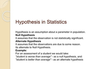
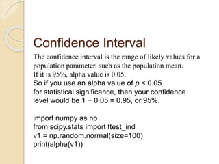
Statistical tests help justify if sample results can be applied to a population. ANOVA compares group means and is preferred over t-tests for 3+ groups. It calculates variation between and within groups to obtain an F-ratio. If the F-ratio exceeds its critical value, the null hypothesis that group means are equal is rejected, showing group means differ significantly. Two-way ANOVA extends this to consider two factors' influence, computing interaction effects between factors.

1. Statistical Significance Tests
Hypothesis
Null Hypothesis
Alternate Hypothesis
T-Test

2. Statistical Significance Test
In statistics, statistical significance means that the result
that was produced has a reason behind it, it was not
produced randomly, or by chance.
SciPy provides us with a module called scipy.stats,
which has functions for performing statistical
significance tests.

3. Hypothesis in Statistics
Hypothesis is an assumption about a parameter in population.
Null Hypothesis
It assumes that the observation is not statistically significant.
Alternate Hypothesis
It assumes that the observations are due to some reason.
Its alternate to Null Hypothesis.
Example:
For an assessment of a student we would take:
"student is worse than average" - as a null hypothesis, and:
"student is better than average" - as an alternate hypothesis

4. Examples of NULL Hypothesis
For most tests, the null hypothesis is that there is no
relationship between your variables of interest or that there is
no difference among groups.
The p value, or probability value, tells you how likely it is that
your data could have occurred under the null hypothesis.
The p value is a proportion: if your p value is 0.05, that
means that 5% of the time you would see a test statistic for
NULL hypothesis
P values are usually automatically calculated by your
statistical program using tables for estimating

5. One tailed test
When our hypothesis is testing for one side of the
value only, it is called "one tailed test".
Example:
For the null hypothesis:
"the mean is equal to k",
we can have alternate hypothesis:
"the mean is less than k", or:
"the mean is greater than k"

6. Two tailed test
When our hypothesis is testing for both side of the
values.
Example:
For the null hypothesis:
"the mean is equal to k",
we can have alternate hypothesis:
"the mean is not equal to k"
In this case the mean is less than, or greater than k,
and both sides are to be checked.

7. Alpha Value and P Value
P value and alpha values are compared to establish
the statistical significance.
Alpha value is the level of significance.
Example:
How close to extremes the data must be for null
hypothesis to be rejected.
It is usually taken as 0.01, 0.05, or 0.1.
P value
P value tells how close to extreme the data actually is.
If p value <= alpha we reject the null hypothesis and
say that the data is statistically significant. otherwise
we accept the null hypothesis.

8. Confidence Interval
The confidence interval is the range of likely values for a
population parameter, such as the population mean.
If it is 95%, alpha value is 0.05.
So if you use an alpha value of p < 0.05
for statistical significance, then your confidence
level would be 1 − 0.05 = 0.95, or 95%.
import numpy as np
from scipy.stats import ttest_ind
v1 = np.random.normal(size=100)
print(alpha(v1))

9. T-Test :: two tailed test
import numpy as np
from scipy.stats import ttest_ind
v1 = np.random.normal(size=100)
v2 = np.random.normal(size=100)
res = ttest_ind(v1, v2)
print(res)
#p-value
res = ttest_ind(v1, v2).pvalue
print(res)
T-tests are used to determine
if there is significant deference
between means of two
variables. and lets us know if
they belong to the same
distribution.

10. You find two different species of irises growing in a
garden and measure 25 petals of each species. You
can test the difference between these two groups
using a t test and null and alterative hypotheses.
The null hypothesis (H0) is that the true difference
between these group means is zero.
The alternate hypothesis (Ha) is that the true
difference is different from zero.

11. A t test can only be used when comparing the means of two groups
( pairwise comparison).
To compare more than two groups, or to do multiple pairwise
comparisons, use an ANOVA test
Parametric test : T-test (comparison tests), regression tests, and
correlation tests.
stricter requirements, common assumptions
and so are able to make stronger inferences from the data.
Non-parametric tests don’t make as many assumptions about the
data, some common statistical assumptions are violated. However,
the inferences they make aren’t as strong as parametric test
Ex. Wilcoxon Signed-rank test, Chi square test of independence,
Kruskal–Wallis H

12. Most statistical software (R, SPSS, etc.) includes a t test function. This
built-in function will take your raw data and calculate the t value. It will
then compare it to the critical value, and calculate a p-value.

13. ANOVA – Analysis of Variance
The two fundamental concepts in inferential statistics
are population and sample. The goal of the inferential
statistics is to infer the properties of a population
based on samples.
Population is all elements in a group whereas sample
means a randomly selected subset of the population.
It is not always feasible or possible to collect
population data so we perform analysis using

14. Statistical Test
It would not be correct to directly apply the sample
analysis results to the entire population.
We need systematic ways to justify the sample
results are applicable to the population. This is
done by statistical tests.
Statistical tests evaluate how likely the sample
results are true representation of the population.
For ex.we want to compare the average weight of
20-year-old people in two different countries, A and
B. Since we cannot collect the population data, we
take samples and perform a statistical test.

15. Assume we are comparing three countries, A, B,
and C. We need to apply a t-test to A-B, A-C and B-
C pairs. As the number of groups increase, this
becomes harder to manage.
In the case of comparing three or more groups,
ANOVA is preferred.
There are two elements of ANOVA:
Variation within each group
Variation between groups

16. Calculation
ANOVA result is based on the F ratio which is calculated as
follows:
F ratio is a measure of the comparison between the variation
between groups and variation within groups.
Variation between groups/ variation within groups
F ratio>1, means of groups are different, individual variation is
less

17. F values above 1 indicates that at least one of the groups is
different than the others.
p-value is very small which indicates the results are statistically
significant (i.e. not generated due to random chance). Typically,
results with p-values less than 0.05 are assumed to be
statistically significant.
Df is degrees of freedom. First line is for the variation between
groups and the second line is for the variation within groups
which are calculated as follows:
DF for variation between groups= Number of groups -1
DF for variation within group= Total no of observations- Total no
of groups

18. Types
one-way ANOVA test :: compares the means of
three or more groups based on one independent
variable.
two-way ANOVA test :: compares three or more
groups based on two independent variables.

19. The basic idea behind a one-way ANOVA is to take
independent random samples from each group, then
compute the sample means for each group. After that
compare the variation of sample means among the
groups to the variation within the groups. Finally, make
a decision based on a test statistic, whether the means
of the groups are all equal or not.
For ex. annual salary of graduates : mean is affected
by subject of study
If there are 6 subjects, every subject has a group,
mean of every group is affecting mean of annual salary

20. Sum of Squares (SS)
The total amount of variability comes from two possible
sources, namely:
1. Difference among the groups, called treatment (TR)
2. Difference within the groups, called error (E)
F score= Variation between groups/ variation within groups =
Sum of squares between groups / sum of squares within group=
SSTR / SSE = (SSb/ d.f.TR) / (SSw/ d.f.E) = (SSb/(c-1) /
(SSw/(n-c)
d.f. (SSTO) = d.f. (SSTR) + d.f. (SSE) = ( c-1 ) + (n-c) = n-1
Null Hypothesis – There is no significant difference among
the groups
Alternate Hypothesis – There is a significant difference
among the groups

21. Yi, mean of ith group, ni no of observations in ith group
Y mean , yij jth observation, k total no of groups, N total no of
samples

22. ANOVA TEST PROCEDURE
Setup null and alternative hypothesis where null
hypothesis states that there is no significant
difference among the groups. And alternative
hypothesis assumes that there is a significant
difference among the groups.
Calculate F-ratio and probability of F.
Compare p-value of the F-ratio with the established
alpha or significance level.
If p-value of F is less than 0.5 then reject the null
hypothesis.
If null hypothesis is rejected, conclude that mean of
groups are not equal.

23. Assumptions
•We can obtain observations randomly and
independently from the population defined by the
factor levels.
•The data for every level of the factor is distributed
generally.
•Case Independent: The sample cases must be
independent of each other.
•Variance Homogeneity: Homogeneity signifies that
the variance between the group needs to be around
equal. (Histogram and normality score for
distribution)

24. Case Study one way ANOHA
The idea is similar to conducting a survey. We take three
different groups of ten randomly selected students (all of
the same age) from three different classrooms. Each
classroom was provided with a different environment for
students to study.
Objective is to assess statistical significance of factor.
A – constant sound, B- variable sound
C- No sound

25. Manual Calculation
Clas
s
Out Of 10 test Scores Me
an
A 7 9 5 8 6 8 6 10 7 4 ?
B 4 3 6 2 7 5 5 4 1 3 ?
C 6 1 3 5 3 4 6 5 7 3 ?
Grand
Mean
?
SSb=54.6
SSw=90.1
d.f.b=2
d.f.w.=27
F score= 8.18
Alpha=0.05
P-value=0.001
F-Critical = 3.35
This F-statistic calculated here
is compared with the F-critical
value for making a conclusion.
F0.05
2,27 = ? F table

26. 1.9 3.61 36.1
-1.1 1.21 12.1
-0.8 0.64 6.4
54.6
7 0 0
9 2 4
5 -2 4
8 1 1
6 -1 1
8 1 1
6 -1 1
10 3 9
7 0 0
4 7 -3 9

27. if the value of the calculated F-statistic is more
than the F-critical value (for a specific
α/significance level), then we reject the null
hypothesis and can say that the treatment had a
significant effect.
If the F-statistic lands in the critical region, we
can conclude that the means are significantly
different and we reject the null hypothesis.
How do we decide that these three groups
performed differently because of the different
situations and not merely by chance?
In a statistical sense, how different are these
three samples from each other?
What is the probability of group A students
performing so differently than the other two

28. Summary
ANOVA is a method to determine if the mean of groups
are different.
In inferential statistics, we use samples to infer
properties of populations. Statistical tests like ANOVA
help us justify if sample results are applicable to
populations.
The difference between t-test and ANOVA is that t-test
can only be used to compare two groups where ANOVA
can be extended to three or more groups.
ANOVA can also be used in feature selection process of
machine learning. The features can be compared by
performing an ANOVA test and similar ones can be
eliminated from the feature set.

29. Case Study 2 way ANOVA
Example: Suppose you want to
determine whether the brand of
laundry detergent used and the
temperature affects the amount
of dirt removed from your
laundry.

30. Two-Way ANOVA
cold
Warm hot
4 7 10
5 9 12
6 8 11
Super 5 12 9
6 13 12
6 15 13
4 12 10
Best 4 12 13
Replica r=4, a=2,b=3, total samples=24

31. Cold Warm Hot Mean
Combin
4 7 10
5 9 12
6 8 11
5 12 9
Super 5 9 10 8
6 13 12
6 15 13
4 12 10
4 12 13
Best 5 13 12 10
Mean T 5 11 11 9

32. Steps for 2 WAY ANOHA
Calculate SS between, SS Within , and interaction of factors
D.F. within= (r-1)*a*b = 3*2*3=18
4 4-5 (-1)^2
5 5-5 (0)^2
6 6-5 (1)^2
5 5-5 (0)^2
5
SS within = sum of squares
Mean square= SS within (38) /18 =2.111

33. SS between
4*3[(8-9)²+(10-9)²] SS (detergent)
2-1=1 DF(detergent)
Mean square(detergent) = 24/1
SS(temperature) 4*2*[(5 − 9)² + (11 − 9)² + (11 − 9)²]
DF(temperature) 3-1=2
Mean square (temp) 192/2
SS(interaction)=4* {(5-8-5+9)^2+(9-8-11+9)^2+(10-8-
11+9)^2+(5-10-5+9)^2+(12-10-11+9)^2+(12-10-11+9)^2
DF(interaction)=(a-1)*(b-1)=2
Mean square(interaction)=16/2
Three F scores are calculated

34. Multi-variate ANOVA (MANOVA)
4-8 yrs 8-13 yrs 13-17 yrs
A 6 4 7
A 5 5 6
B 1 4 6
B 3 5 8
History Maths
A 7 3
A 9 1
B 10 5
B 7 9
Generate ANOVA table for Individual factor and compare the
conclusion or Null Hypothesis testing for both.

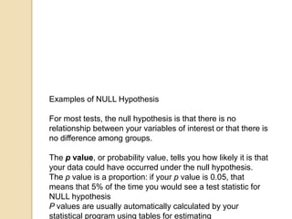
35. Python code
import pandas as pd
import random
# read original dataset
student_df = pd.read_csv('students.csv')
# filter the students who are graduated
graduated_student_df = student_df[student_df['graduated'] == 1]
# random sample for 500 students
unique_student_id = list(graduated_student_df['stud.id'].unique())
random.seed(30) # set a seed so that everytime we will extract same
samplesample_student_id = random.sample(unique_student_id, 500)
sample_df =
graduated_student_df[graduated_student_df['stud.id'].isin(sample_student_i
d)].reset_index(drop=True)

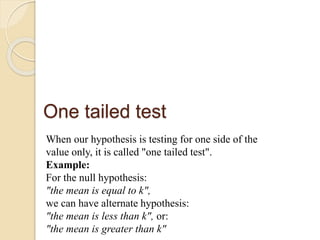
36. # two variables of interestsample_df = sample_df[['major', 'salary']]
groups = sample_df.groupby('major').count().reset_index()
groups
# calculate ratio of the largest to the smallest sample standard deviation
ratio = sample_df.groupby('major').std().max() /
sample_df.groupby('major').std().min()ratio
Homogeneity of variance Assumption Check
The ratio of the largest to the smallest sample standard deviation is 1.67. T It
should be less than the threshold of 2 which is homogeneity of variance check.

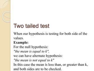
37. # Create ANOVA backbone table
data = [['Between Groups', '', '', '', '', '', ''], ['Within
Groups', '', '', '', '', '', ''], ['Total', '', '', '', '', '', '']]
anova_table = pd.DataFrame(data, columns =
['Source of Variation', 'SS', 'df', 'MS', 'F', 'P-value',
'F crit'])
anova_table.set_index('Source of Variation',
inplace = True)
Source
of
variation
SS DF MS F P-
value
F-Crit

38. # calculate SSTR and update anova table
x_bar = sample_df['salary'].mean()
SSTR = sample_df.groupby('major').count() *
(sample_df.groupby('major').mean() - x_bar)**2
anova_table['SS']['Between Groups'] = SSTR['salary'].sum()
# calculate SSE and update anova table
SSE = (sample_df.groupby('major').count() - 1) *
sample_df.groupby('major').std()**2
anova_table['SS']['Within Groups'] = SSE['salary'].sum()

39. # calculate SSTR and update anova table
SSTR = SSTR['salary'].sum() + SSE['salary'].sum()
anova_table['SS']['Total'] = SSTR
# update degree of freedom
anova_table['df']['Between Groups'] =
sample_df['major'].nunique() – 1
anova_table['df']['Within Groups'] = sample_df.shape[0] -
sample_df['major'].nunique()
anova_table['df']['Total'] = sample_df.shape[0] – 1
# calculate MS
anova_table['MS'] = anova_table['SS'] / anova_table['df']

40. # calculate F F = anova_table['MS']['Between Groups'] /
anova_table['MS']['Within Groups']
anova_table['F']['Between Groups'] = F
# p-value
anova_table['P-value']['Between Groups'] = 1 - stats.f.cdf(F,
anova_table['df']['Between Groups'], anova_table['df']['Within
Groups'])

41. # F critical
alpha = 0.05
# possible types "right-tailed, left-tailed, two-tailed“
tail_hypothesis_type = "two-tailed“
if tail_hypothesis_type == "two-tailed":
alpha /= 2
anova_table['F crit']['Between Groups'] = stats.f.ppf(1-alpha,
anova_table['df']['Between Groups'], anova_table['df']['Within
Groups'])
# Final ANOVA Table
anova_table

42. Tutorial Question
4-8 years 8-13 yeras 13-17 years
A 6 4 7
5 5 6
5 6 10
2 9 8
4 8 9
B 1 4 6
3 5 8
2 6 4
1 7 7
2 3 5