Download as PDF, PPTX

![Analytical approach (AA)
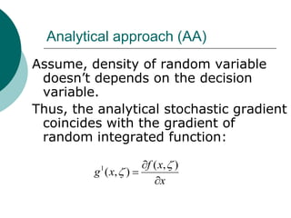
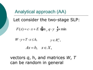
The stochastic analytical gradient is defined as
g 1 ( x, ) c T u *
by the a set of solutions of the dual problem
(h T x)T u* maxu [(h T x)T u | u W T q 0, u m
]](https://image.slidesharecdn.com/lecture3-100818113259-phpapp01/85/Stochastic-Differentiation-9-320.jpg)

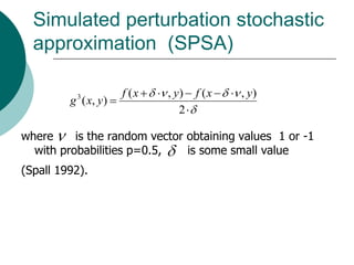
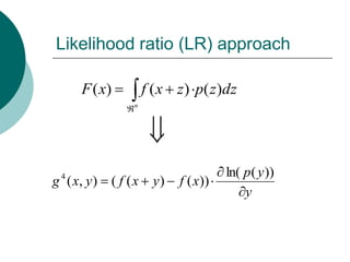
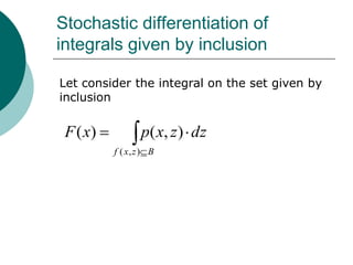

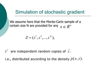

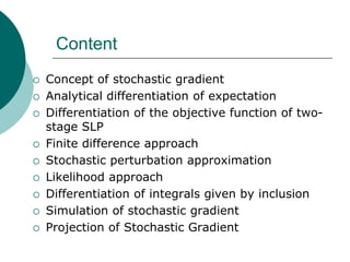
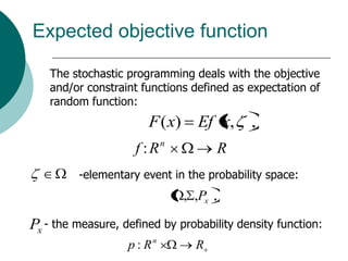
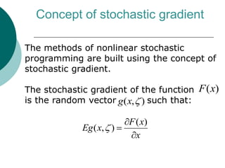
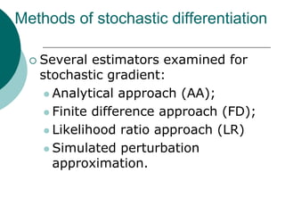
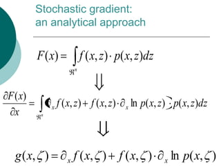
The document discusses stochastic differentiation, focusing on the concept of stochastic gradient in nonlinear stochastic programming. It explores various methods for obtaining stochastic gradients, including analytical, finite difference, simulated perturbation, and likelihood ratio approaches. Additionally, it covers simulation techniques for estimating objective functions and gradients using Monte Carlo samples.