Download as PDF, PPTX
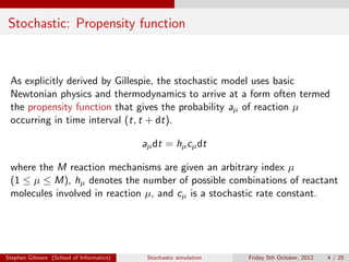


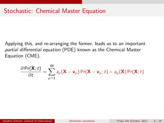


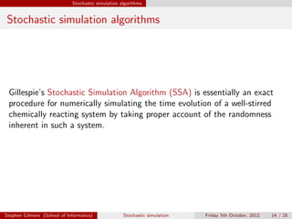
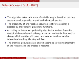
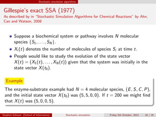


The document discusses the stochastic simulation algorithm (SSA) for modeling chemical reactions. It explains that molecular reactions are inherently random processes. The SSA was developed by Gillespie to take into account this randomness by simulating reaction times and species populations. The algorithm works by choosing reaction times and events based on propensity functions derived from statistical thermodynamics. It provides an exact numerical simulation of a well-stirred chemically reacting system.


![Digital Signal Processing[ECEG-3171]-Ch1_L03](https://cdn.slidesharecdn.com/ss_thumbnails/dspl3-180427094423-thumbnail.jpg?width=640&height=640&fit=bounds)