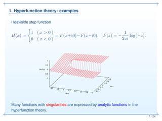
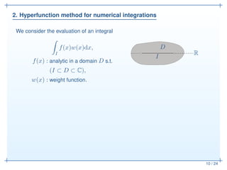
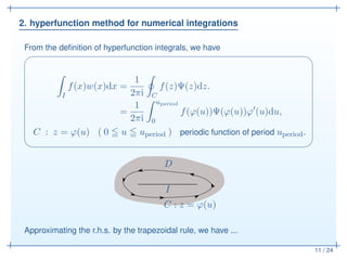
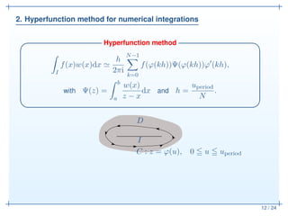
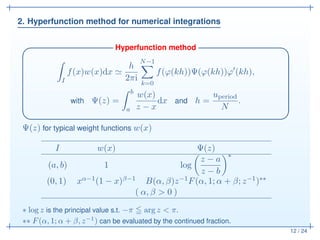
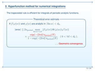
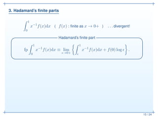
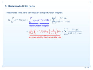
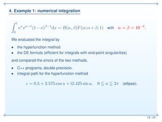
The document discusses the application of hyperfunction theory, a generalized function theory based on complex analysis, to numerical integration methods. It elaborates on techniques for numerical integrations and Hadamard's finite parts, providing examples and demonstrating the efficiency of the hyperfunction method, particularly for integrals with end-point singularities. The findings suggest that hyperfunction theory can greatly enhance various scientific computations.

1. 1 / 24
An Application of the Hyperfunction Theory to Numerical Integration
ECMI2016
∗Hidenori Ogata (The University of Electro-Communications, Japan)
Hiroshi Hirayama (Kanagawa Institute of Technology, Japan)
17 June 2016

2. Contents
2 / 24
✓ ✏
We show an application of the hyperfunction theory, a generalized function
theory based on complex analysis, to numerical computations, in particular,
to numerical integrations.
✒ ✑

3. Contents
2 / 24
✓ ✏
We show an application of the hyperfunction theory, a generalized function
theory based on complex analysis, to numerical computations, in particular,
to numerical integrations.
✒ ✑
1. Hyperfunction theory
2. Hyperfunction method for numerical integrations
3. Hyperfunction method for Hadamard’s finite parts
4. Numerical examples
5. Summary

4. Contents
3 / 24
1. Hyperfunction theory
2. Hyperfunction method for numerical integrations
3. Hyperfunction method for Hadamard’s finite parts
4. Numerical examples
5. Summary

5. 1. Hyperfunction theory (M. Sato, 1958)
4 / 24
b
a
φ(x)δ(x)dx = φ(0).
1
2πi C
φ(z)
z
dz = φ(0).
( a < 0 < b )
Dirac delta function Cauchy integral formula
O
C

6. 1. Hyperfunction theory (M. Sato, 1958)
4 / 24
b
a
φ(x)δ(x)dx = φ(0).
1
2πi C
φ(z)
z
dz = φ(0).
( a < 0 < b )
Dirac delta function Cauchy integral formula
O
C
Oa b
1
2πi C
φ(z)
z
dz = −
1
2πi
b
a
φ(x)
1
x + i0
−
1
x − i0
dx.

7. 1. Hyperfunction theory (M. Sato, 1958)
4 / 24
b
a
φ(x)δ(x)dx = φ(0).
1
2πi C
φ(z)
z
dz = φ(0).
( a < 0 < b )
Dirac delta function Cauchy integral formula
O
C
Oa b
b
a
φ(x)δ(x)dx =
1
2πi C
φ(z)
z
dz = −
1
2πi
b
a
φ(x)
1
x + i0
−
1
x − i0
dx.
∴ δ(x) = −
1
2πi
1
x + i0
−
1
x − i0
.

8. 1. Hyperfunction theory
5 / 24
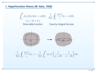
Hyperfunction theory (M. Sato, 1958)✓ ✏
• A generalized function theory based on complex analysis.
• A hyperfunction f(x) on an interval I is the difference of the boundary
values of an analytic function F(z).
f(x) = [F(z)] ≡ F(x + i0) − F(x − i0).
F(z) : the defining function of the hyperfunction f(x)
analytic in D I,
where D is a complex neighborhood of the interval I.
✒ ✑
D
I
R

9. 1. Hyperfunction theory: examples
6 / 24
• Dirac delta function
δ(x) = −
1
2πiz
= −
1
2πi
1
x + i0
−
1
x − i0
.
• Heaviside step function
H(x) =
1 ( x > 0 )
0 ( x < 0 )
= −
1
2πi
{log(−(x + i0)) − log(−(x − i0))} .
∗ log z is the principal value s.t. −π ≦ arg z < π
• Non-integral powers
x+
α
=
xα ( x > 0 )
0 ( x < 0 )
= −
(−(x + i0))α − (−(x − i0))α
2i sin(πα)
(α ∈ Z const.).
∗ zα
is the principal value s.t. −π ≦ arg z < π.

10. 1. Hyperfunction theory: examples
7 / 24
Heaviside step function
H(x) =
1 ( x > 0 )
0 ( x < 0 )
= F(x+i0)−F(x−i0), F(z) = −
1
2πi
log(−z).
-0.4 -0.2 0 0.2 0.4 0.6 0.8 1Re z
-0.6
-0.4
-0.2
0
0.2
0.4
0.6
Im z
-1
-0.5
0
0.5
1
Re F(z)
The real part of the defining function F(z) = −
1
2πi
log(−z).

11. 1. Hyperfunction theory: examples
7 / 24
Heaviside step function
H(x) =
1 ( x > 0 )
0 ( x < 0 )
= F(x+i0)−F(x−i0), F(z) = −
1
2πi
log(−z).
-0.4 -0.2 0 0.2 0.4 0.6 0.8 1Re z
-0.6
-0.4
-0.2
0
0.2
0.4
0.6
Im z
-1
-0.5
0
0.5
1
Re F(z)
Many functions with singularities are expressed by analytic functions in the
hyperfunction theory.

12. 1. Hyperfunction theory: integral
8 / 24
Integral of a hyperfunction f(x) = F(x + i0) − F(x − i0)✓ ✏
I
f(x)dx ≡ −
C
F(z)dz
C : closed path which encircles I in the positive sense
and is included in D (F(z) is analytic in D I).
✒ ✑
D
C
I
• The integral in independent of the choise of C by the Cauchy integral theorem.

13. Contents
9 / 24
1. Hyperfunction theory
2. Hyperfunction method for numerical integrations
3. Hyperfunction method for Hadamard’s finite parts
4. Numerical examples
5. Summary

14. 2. Hyperfunction method for numerical integrations
10 / 24
We consider the evaluation of an integral
I
f(x)w(x)dx,
f(x) : analytic in a domain D s.t.
(I ⊂ D ⊂ C),
w(x) : weight function.
D
I
R

15. 2. Hyperfunction method for numerical integrations
10 / 24
We consider the evaluation of an integral
I
f(x)w(x)dx,
f(x) : analytic in a domain D s.t.
(I ⊂ D ⊂ C),
w(x) : weight function.
D
I
R
We regard the integrand as a hyperfunction.
✓ ✏
f(x)w(x)χI(x) = −
1
2πi
{f(x + i0)Ψ(x + i0) − f(x − i0)Ψ(x − i0)}
with χI(x) =
1 (x ∈ I)
0 (x ∈ I)
, Ψ(z) =
I
w(x)
z − x
dx.
✒ ✑

16. 2. hyperfunction method for numerical integrations
11 / 24
From the definition of hyperfunction integrals, we have
✓ ✏
I
f(x)w(x)dx =
1
2πi C
f(z)Ψ(z)dz.
=
1
2πi
uperiod
0
f(ϕ(u))Ψ(ϕ(u))ϕ′
(u)du,
C : z = ϕ(u) ( 0 ≦ u ≦ uperiod ) periodic function of period uperiod.
✒ ✑
D
C : z = ϕ(u)
I
Approximating the r.h.s. by the trapezoidal rule, we have ...

17. 2. Hyperfunction method for numerical integrations
12 / 24
Hyperfunction method✓ ✏
I
f(x)w(x)dx ≃
h
2πi
N−1
k=0
f(ϕ(kh))Ψ(ϕ(kh))ϕ′
(kh),
with Ψ(z) =
b
a
w(x)
z − x
dx and h =
uperiod
N
.
✒ ✑
D
C : z = ϕ(u), 0 ≦ u ≦ uperiod
I

18. 2. Hyperfunction method for numerical integrations
12 / 24
Hyperfunction method✓ ✏
I
f(x)w(x)dx ≃
h
2πi
N−1
k=0
f(ϕ(kh))Ψ(ϕ(kh))ϕ′
(kh),
with Ψ(z) =
b
a
w(x)
z − x
dx and h =
uperiod
N
.
✒ ✑
Ψ(z) for typical weight functions w(x)
I w(x) Ψ(z)
(a, b) 1 log
z − a
z − b
∗
(0, 1) xα−1(1 − x)β−1 B(α, β)z−1F(α, 1; α + β; z−1)∗∗
( α, β > 0 )
∗ log z is the principal value s.t. −π ≦ arg z < π.
∗∗ F(α, 1; α + β, z−1
) can be evaluated by the continued fraction.

19. 2. Hyperfunction method for numerical integrations
13 / 24
The trapezoidal rule is efficient for integrals of periodic analytic functions.

20. 2. Hyperfunction method for numerical integrations
13 / 24
The trapezoidal rule is efficient for integrals of periodic analytic functions.
Theoretical error estimate✓ ✏
If f(ϕ(w)) and ϕ(w) are analytic in | Im w| < d0,
|error| ≦ 2uperiod max
Im w=±d
|f(ϕ(w))Ψ(ϕ(w))ϕ′
(w)|
×
exp(−(2πd/uperiod)N)
1 − exp(−(2πd/uperiod)N)
( 0 < ∀d < d0 ).
. . . Geometric convergence.
✒ ✑

21. Contents
14 / 24
1. Hyperfunction theory
2. Hyperfunction method for numerical integrations
3. Hyperfunction method for Hadamard’s finite parts
4. Numerical examples
5. Summary

22. 3. Hadamard’s finite parts
15 / 24
1
0
x−1
f(x)dx ( f(x) : finite as x → 0+ ) . . . divergent!

23. 3. Hadamard’s finite parts
15 / 24
1
0
x−1
f(x)dx ( f(x) : finite as x → 0+ ) . . . divergent!
Hadamard’s finite part✓ ✏
fp
1
0
x−1
f(x)dx ≡ lim
ǫ→0+
1
ǫ
x−1
f(x)dx + f(0) log ǫ .
✒ ✑

24. 3. Hadamard’s finite parts
15 / 24
1
0
x−1
f(x)dx ( f(x) : finite as x → 0+ ) . . . divergent!
Hadamard’s finite part✓ ✏
fp
1
0
x−1
f(x)dx ≡ lim
ǫ→0+
1
ǫ
x−1
f(x)dx + f(0) log ǫ .
✒ ✑
Hadamard’s finite part (n = 1, 2, . . .)✓ ✏
fp
1
0
x−n
f(x)dx
≡ lim
ǫ→+0
1
ǫ
x−n
f(x)dx +
n−2
k=0
ǫk+1−n
k!(k + 1 − n)
f(k)
(0) +
log ǫ
(n − 1)!
f(n−1)
(0) .
✒ ✑

25. 3. Hadamard’s finite parts
16 / 24
Hadamard’s finite parts can be given by hyperfunction integrals.
fp
1
0
x−n
f(x)dx =
1
0
χ(0,1)x−n
f(x)dx
hyperfunction integral
+
n−2
k=0
f(k)
(0)
k!(k + 1 − n)
=
1
2πi C
z−n
f(z) log
z
z − 1
dz
approximated by the trapezoidal rule
+
n−2
k=0
f(k)
(0)
k!(k + 1 − n)

26. Contents
17 / 24
1. Hyperfunction theory
2. Hyperfunction method for numerical integrations
3. Hyperfunction method for Hadamard’s finite parts
4. Numerical examples
5. Summary

27. 4. Example 1: numerical integration
18 / 24
1
0
ex
xα−1
(1−x)β−1
dx = B(α, β)F(α; α+β; 1) with α = β = 10−4
.
We evaluated the integral by
• the hyperfunction method
• the DE formula (efficient for integrals with end-point singularities)
and compared the errors of the two methods.
• C++ programs, double precision.
• integral path for the hyperfunction method
z = 0.5 + 2.575 cos u + i2.425 sin u, 0 ≦ u ≦ 2π (ellipse).

28. 4. Example 1: numerical integrations
19 / 24
-16
-14
-12
-10
-8
-6
-4
-2
0
0 5 10 15 20 25 30
log10(relativeerror)
N
hyperfunction rule
DE rule
relative errors
• the hyperfunction method error = O(0.024N ) (geometric convergence).
• The DE formula does not work for this integral.

29. 4. Example 1: Why the hyperfunction method works well?
20 / 24
integrand
e z
hyperfunction method
• (DE rule) The sampling points accumulate at the singularities.
• (hyperfunction method) The sampling points are distributed on a curve
in the complex plane where the integrand varies slowly.

30. 4. Example 2: Hadamard’s finite part
21 / 24
fp
x
0
x−n
ex
dx =
∞
k=0(k=n−1)
1
k!(k − n + 1)
( n = 1, 2, . . . ).
We computed it by the hyperfunction method.
• C++ program & double precision
• integral path
z =
1
2
+
1
4
ρ +
1
ρ
cos u +
i
4
ρ −
1
ρ
sin u,
0 ≦ u < 2π ( ρ = 10, ellipse ).

31. 4. Example 2: Hadamard’s finite part
22 / 24
-16
-14
-12
-10
-8
-6
-4
-2
0
0 5 10 15 20
log10(relativeerror)
N
n=0
n=1
n=2
n=3
n=4
n=5
the relative errors of the hyperfunction method
n 1 2 3 4 5
error O(0.021N ) O(0.023N ) O(0.018N ) O(0.034N ) O(0.032N )
... geometric convergenc

32. Contents
23 / 24
1. Hyperfunction theory
2. Hyperfunction method for numerical integrations
3. Hyperfunction method for Hadamard’s finite parts
4. Numerical examples
5. Summary

33. 5. Summary
24 / 24
• The hyperfunction theory is a generalized function theory based on complex
analysis.
• The hyperfunction method approximately computes desired integral by
evaluating the complex integrals which define them as hyperfunction
integrals
• Numerical examples show that the hyperfunction method is efficient for
integral with end-point singularities.

34. 5. Summary
24 / 24
• The hyperfunction theory is a generalized function theory based on complex
analysis.
• The hyperfunction method approximately computes desired integral by
evaluating the complex integrals which define them as hyperfunction
integrals
• Numerical examples show that the hyperfunction method is efficient for
integral with end-point singularities.
functions with singularities
(poles, discontinuities,
delta functions, ...)
←−←−←−
hyperfunction
analytic
functions

35. 5. Summary
24 / 24
• The hyperfunction theory is a generalized function theory based on complex
analysis.
• The hyperfunction method approximately computes desired integral by
evaluating the complex integrals which define them as hyperfunction
integrals
• Numerical examples show that the hyperfunction method is efficient for
integral with end-point singularities.
functions with singularities
(poles, discontinuities,
delta functions, ...)
←−←−←−
hyperfunction
analytic
functions
We expect that we can apply the hyperfunction theory to a wide range of
scientific computations.
!
Gracias!