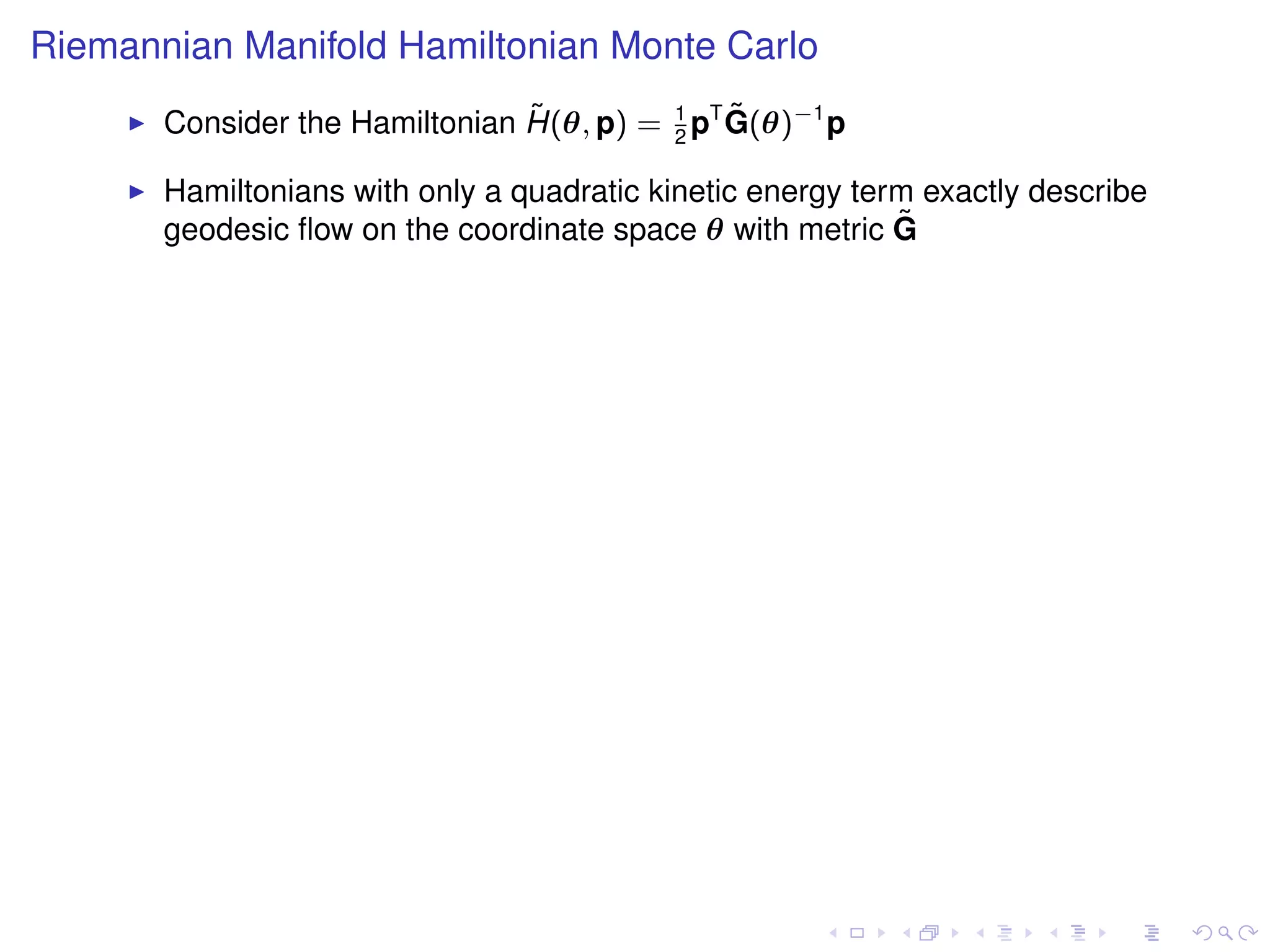
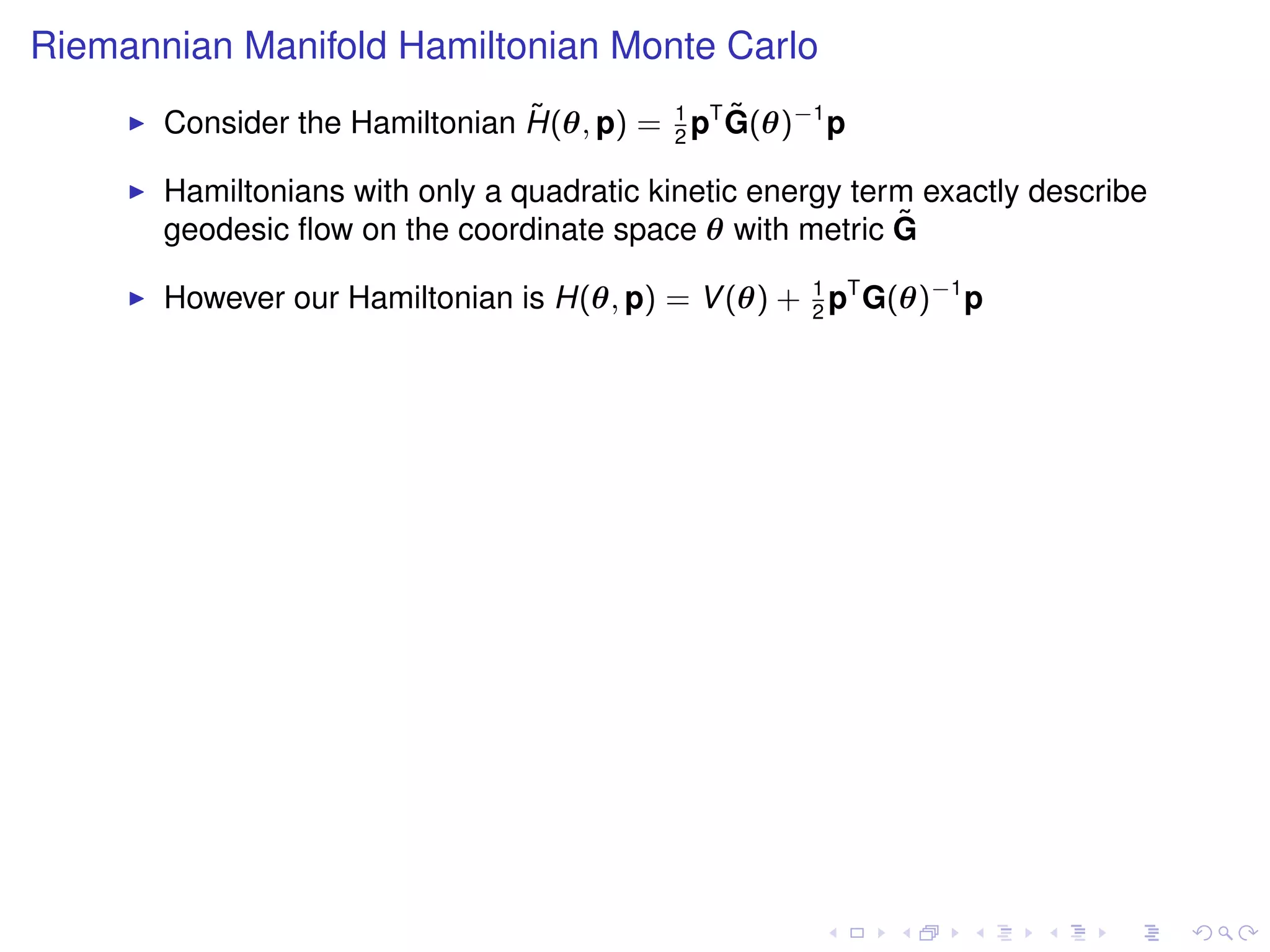
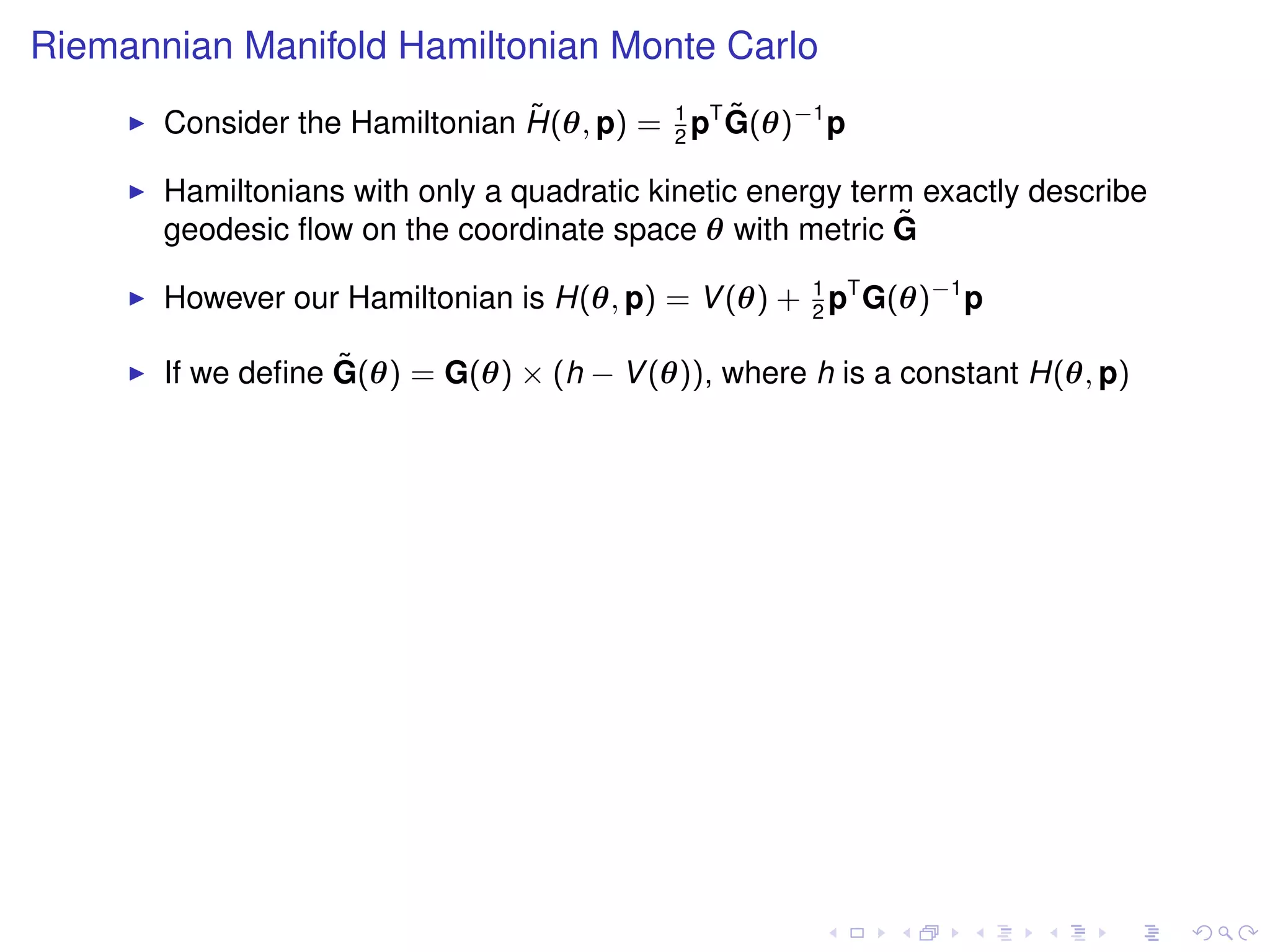
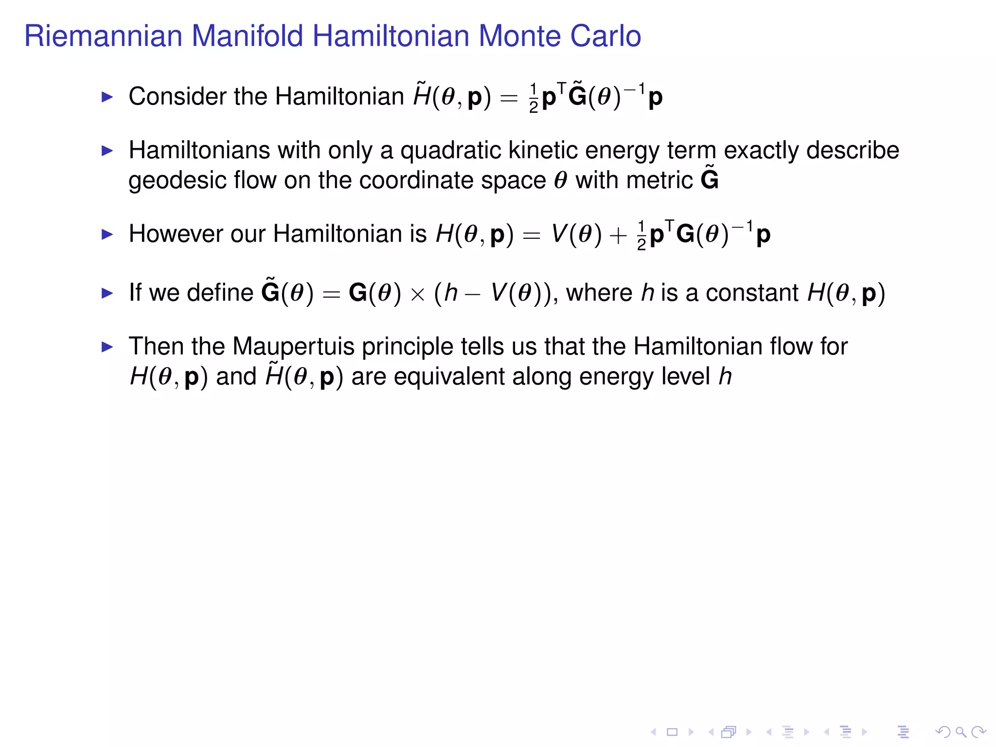
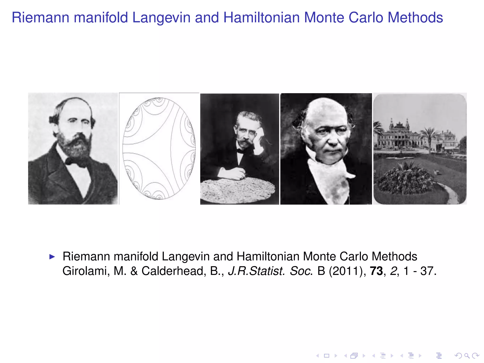
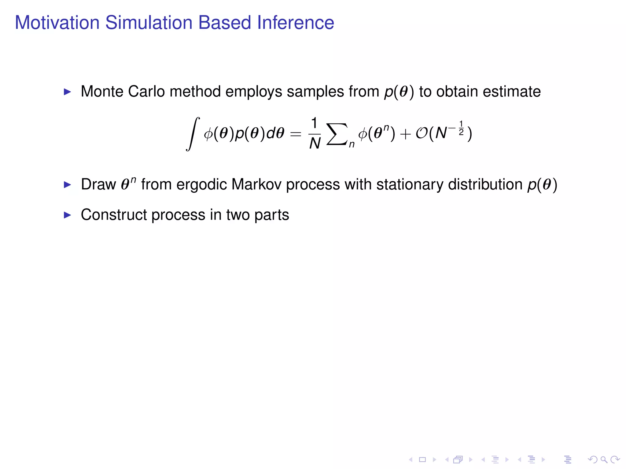
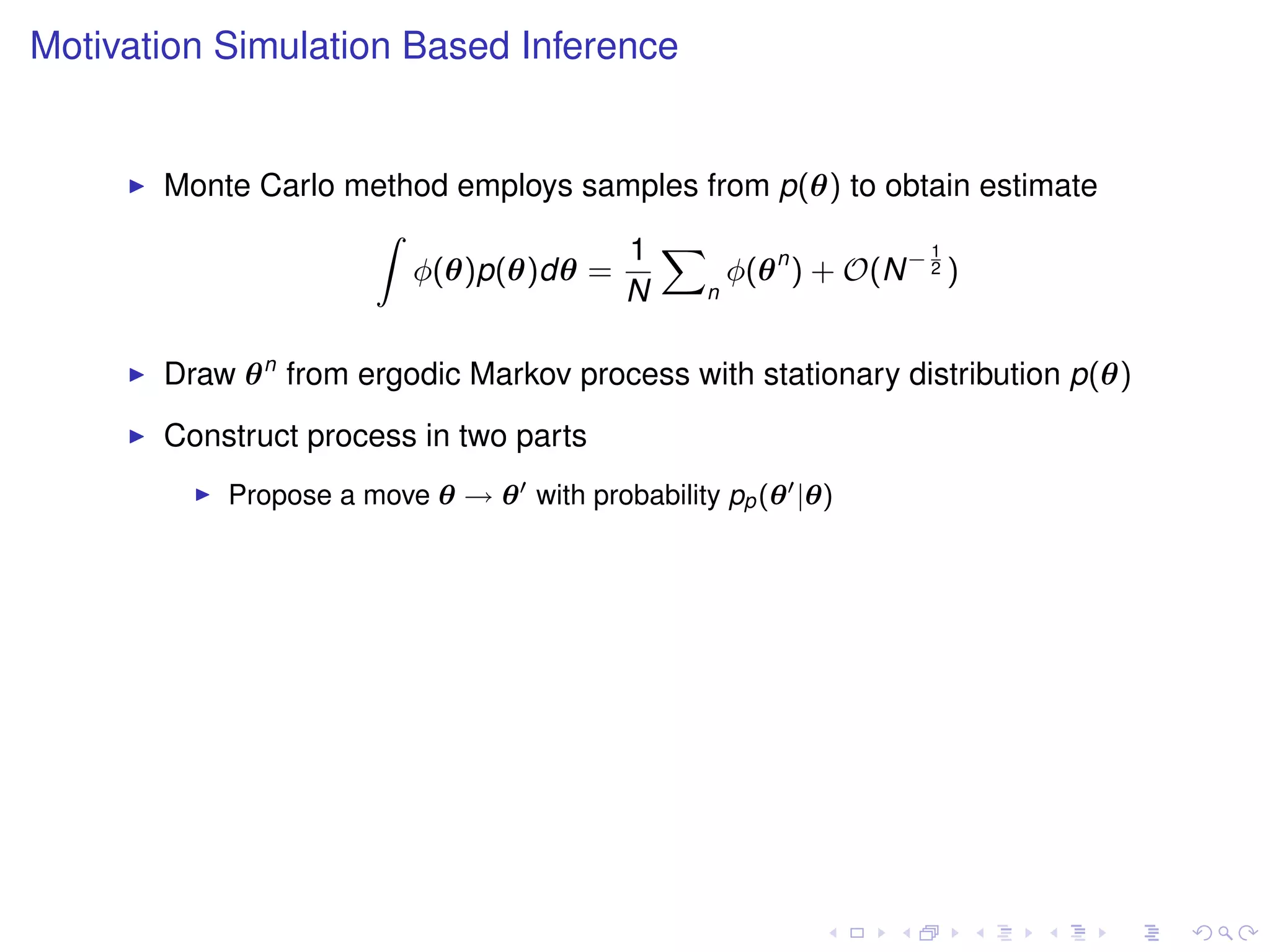
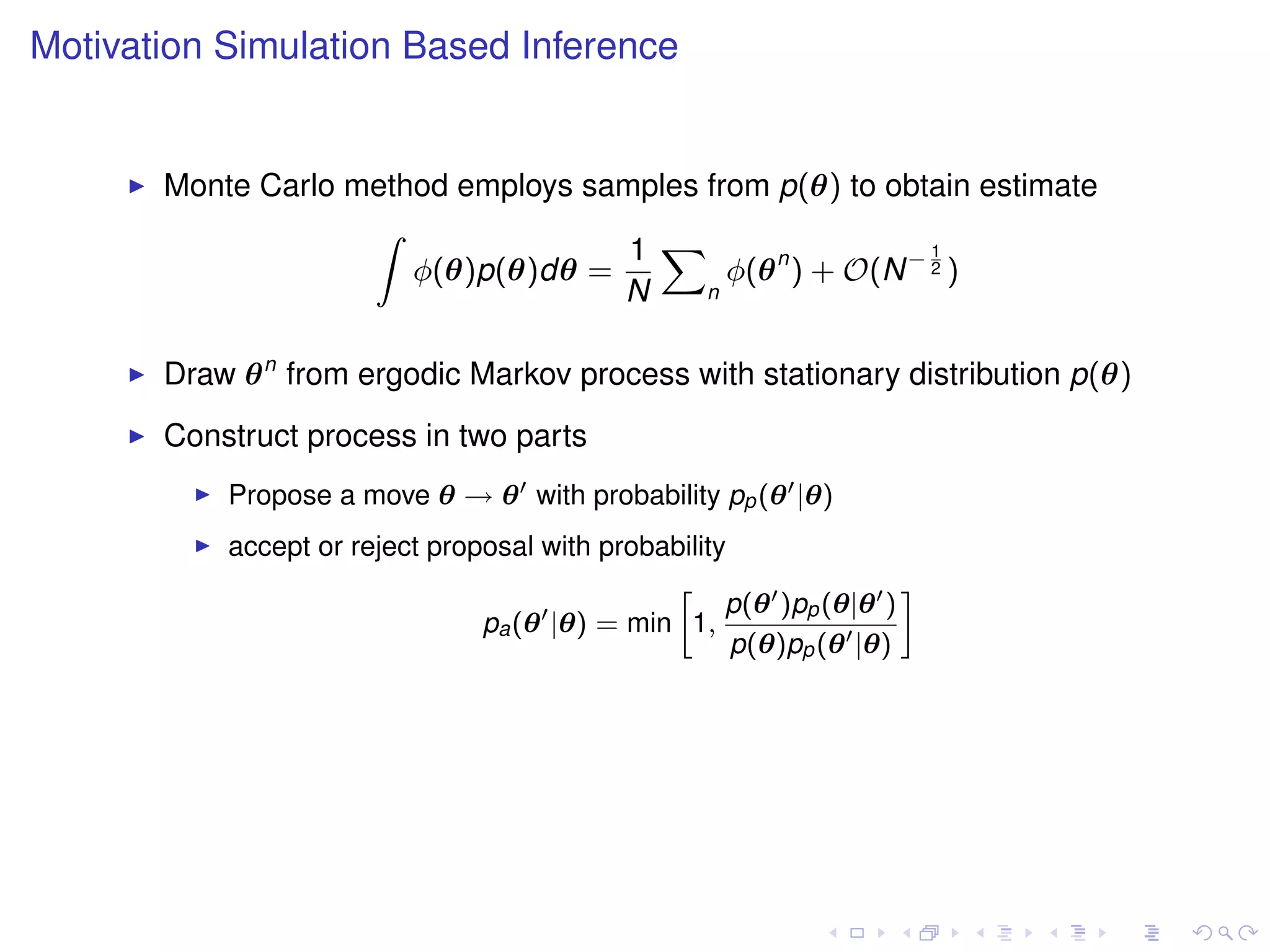
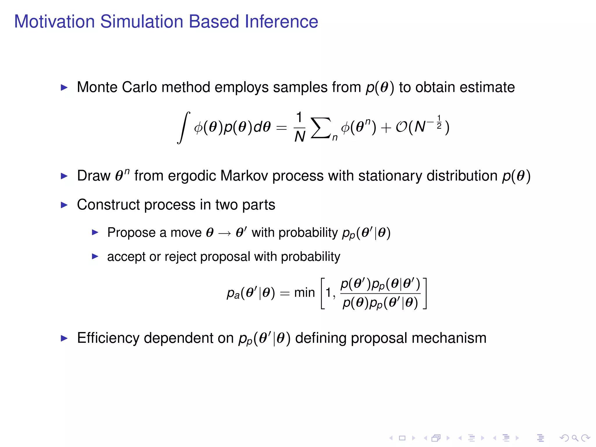
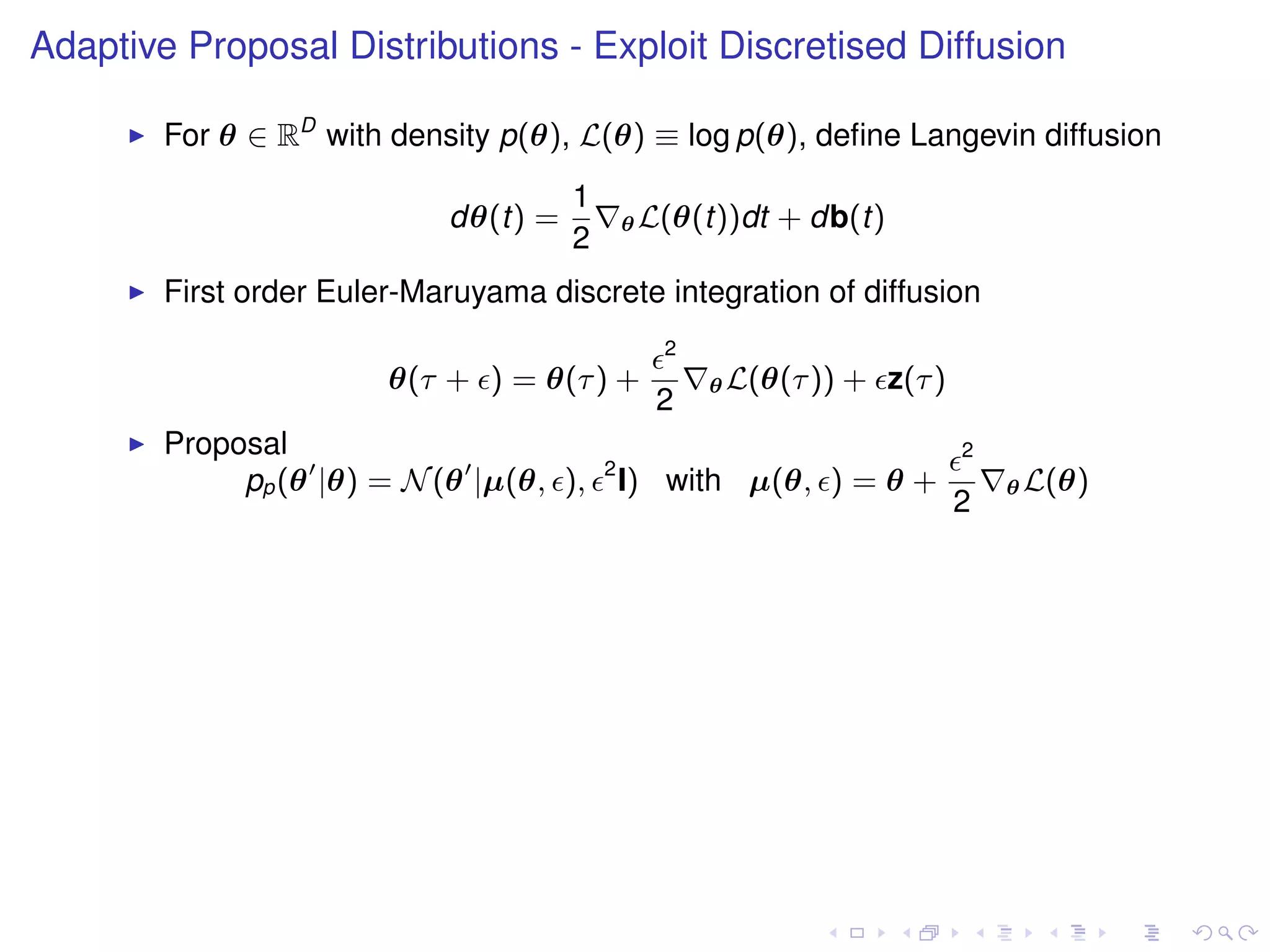
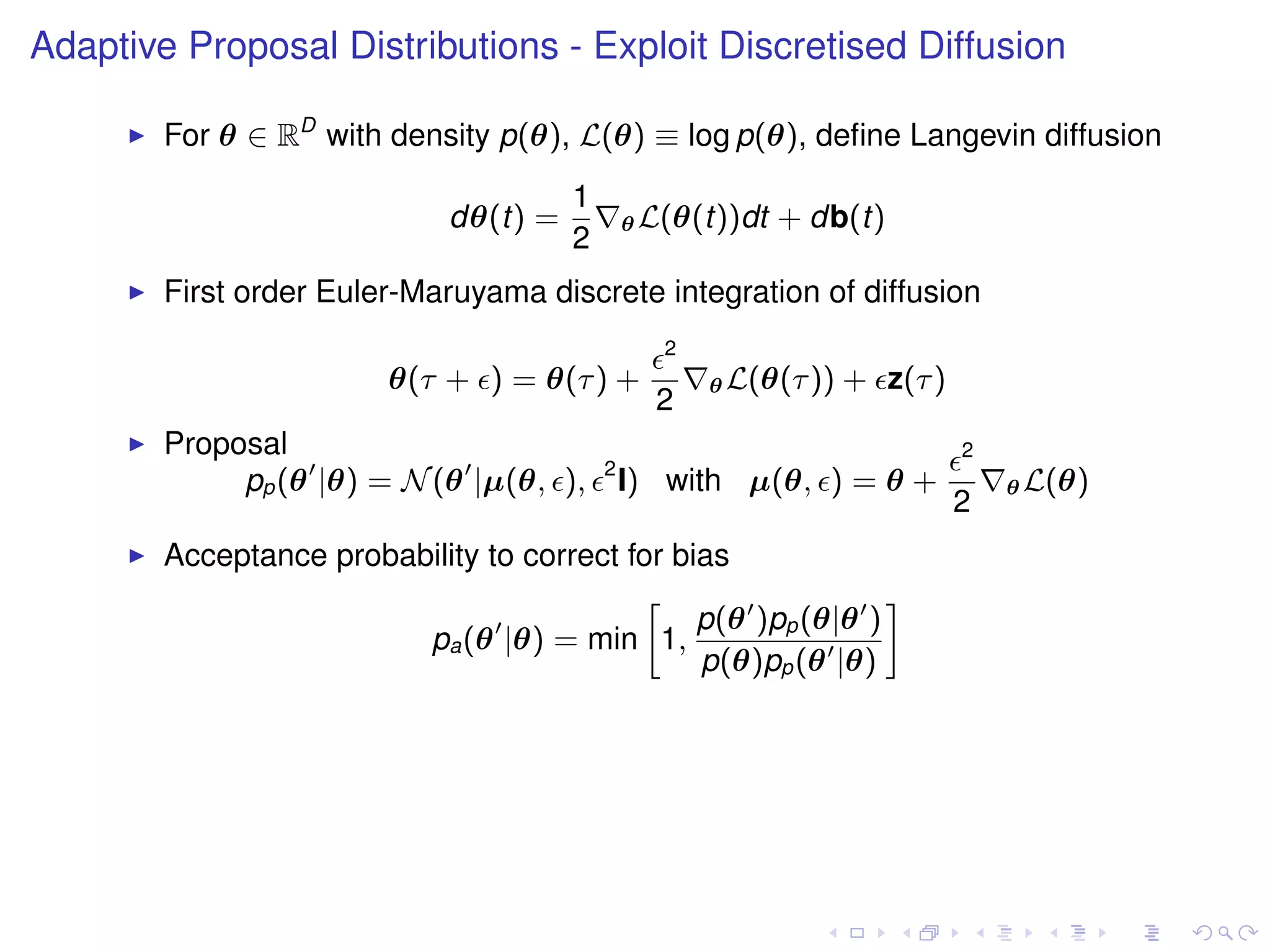
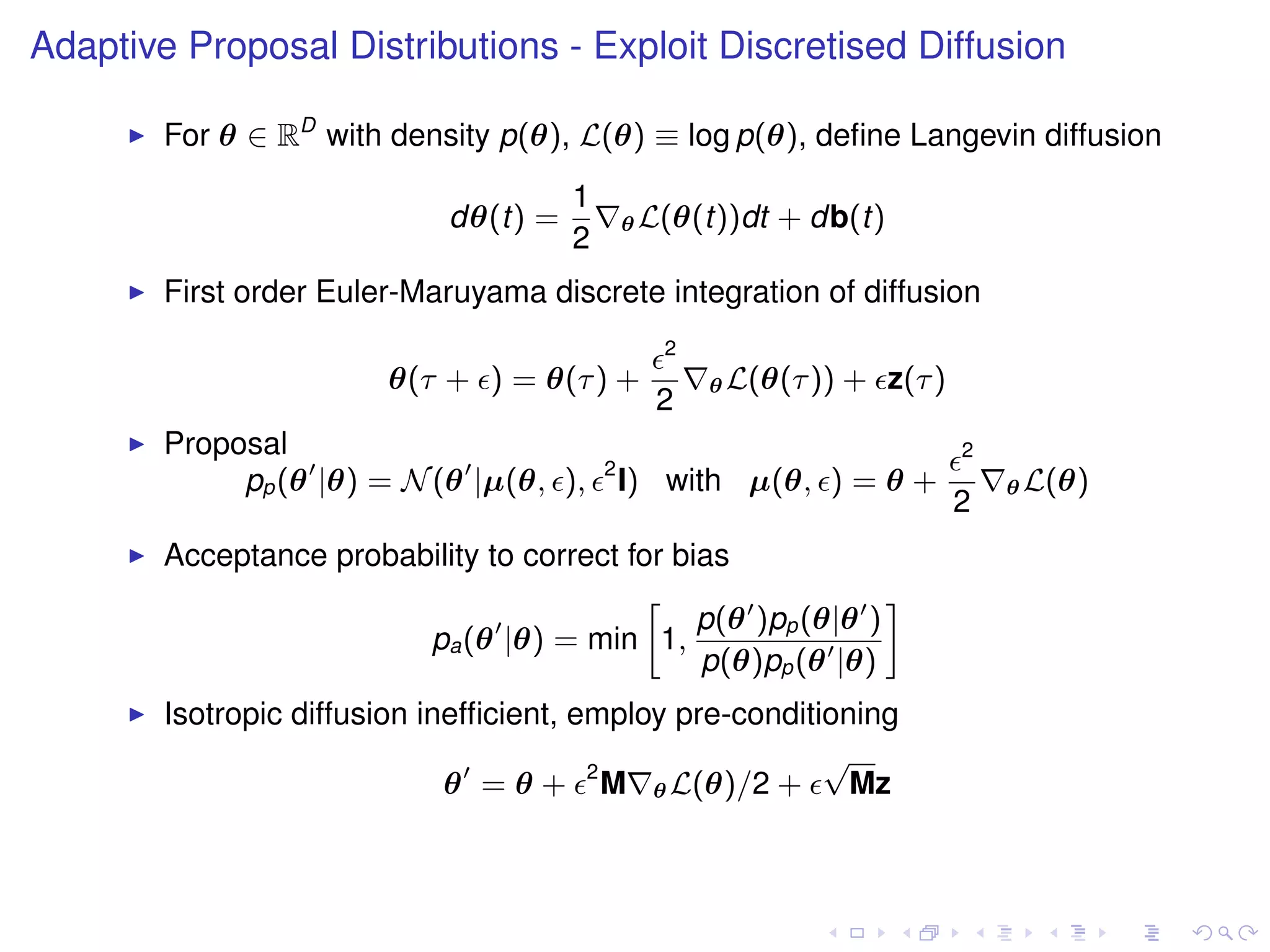
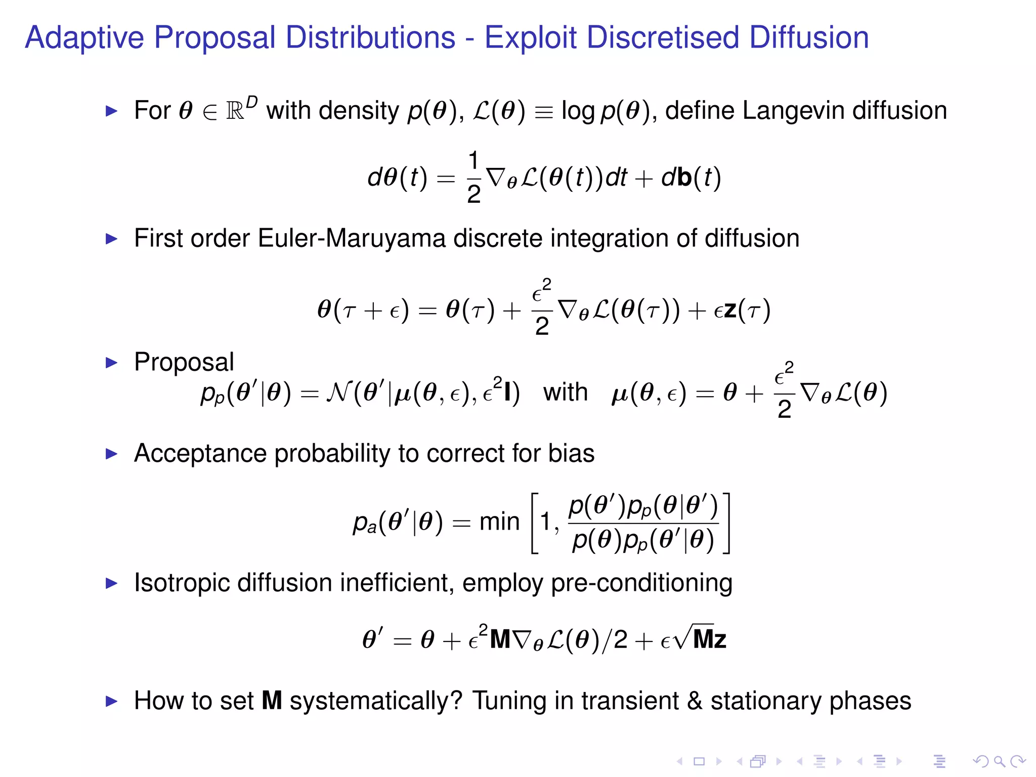
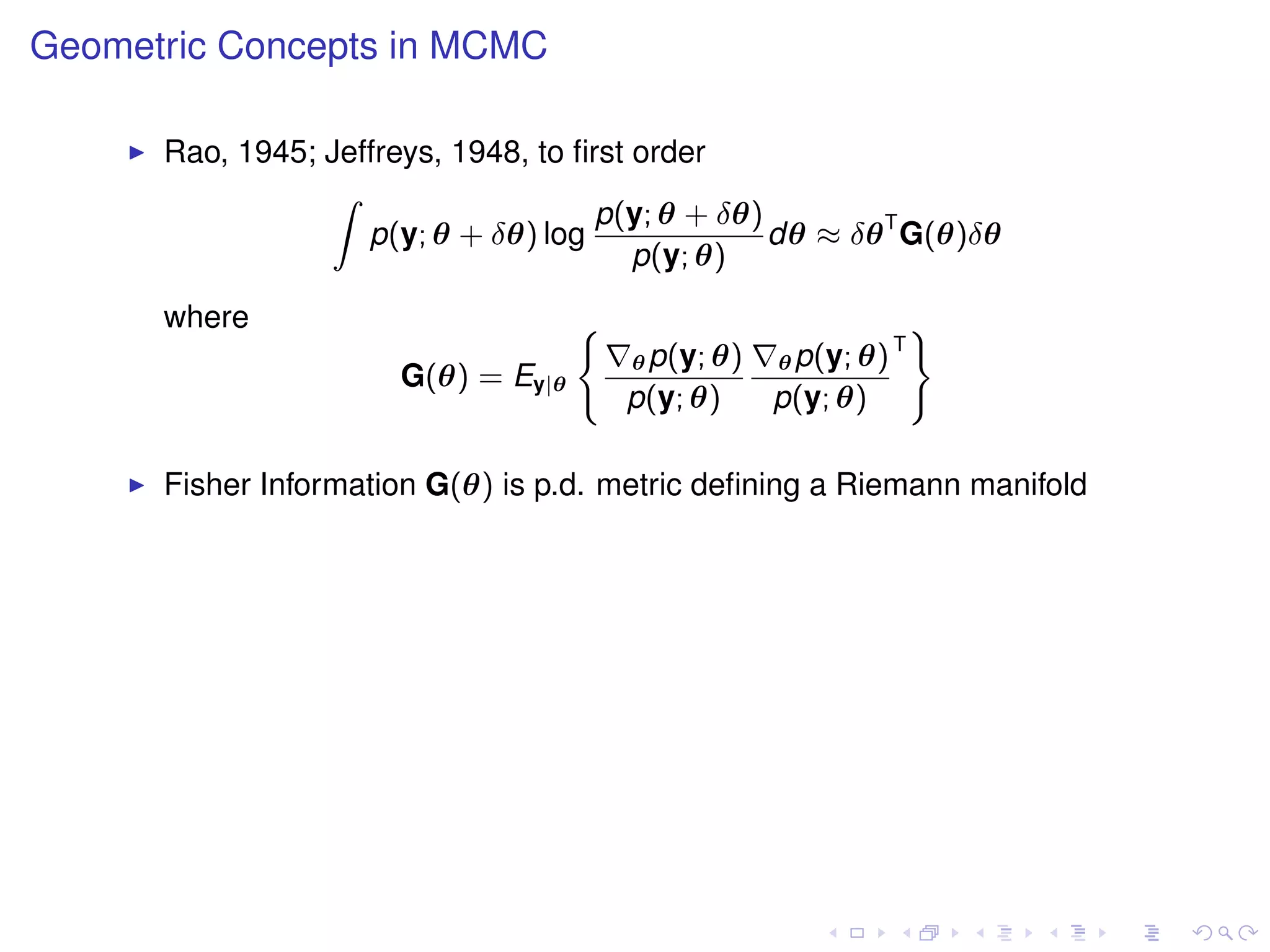
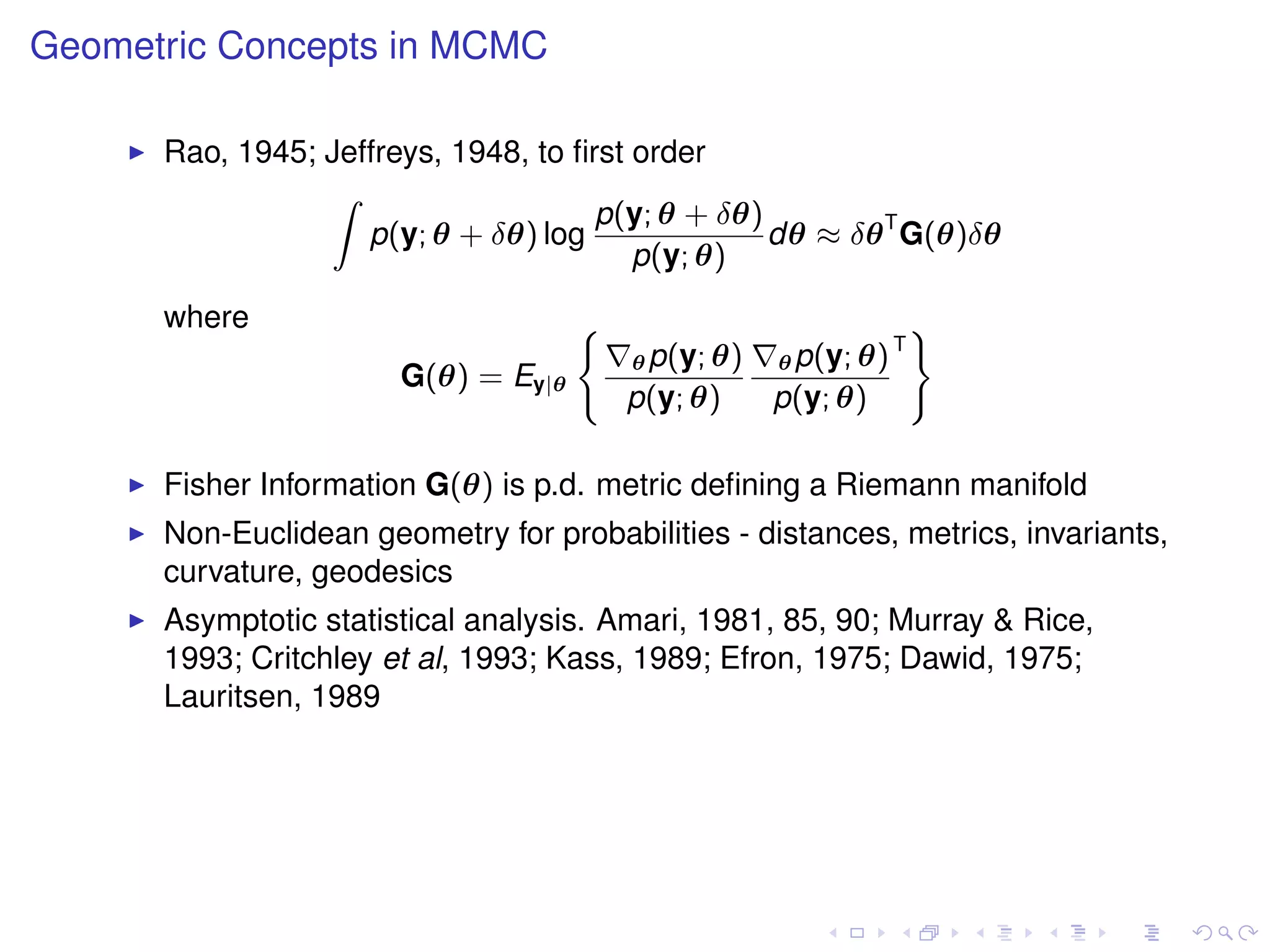
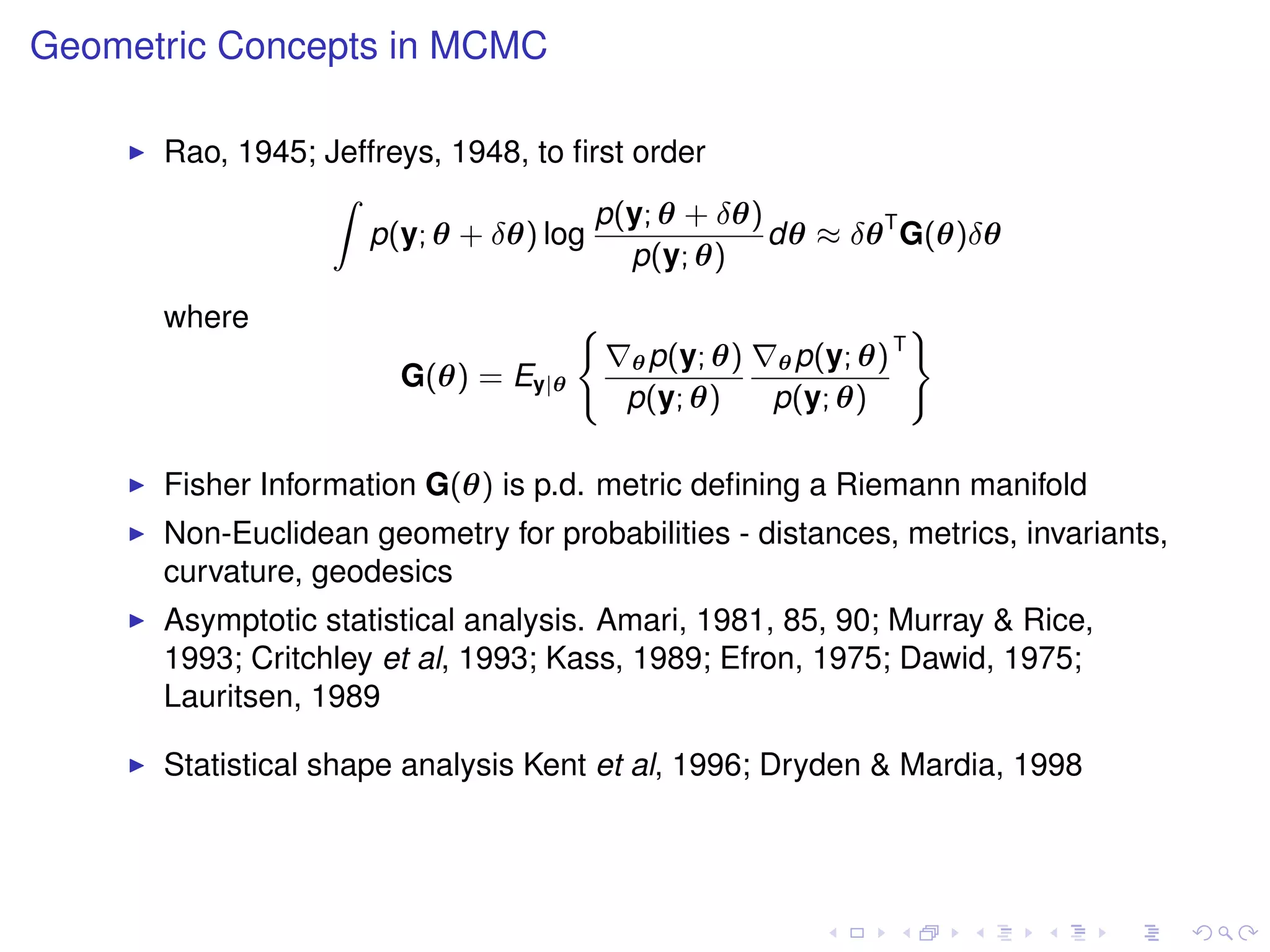
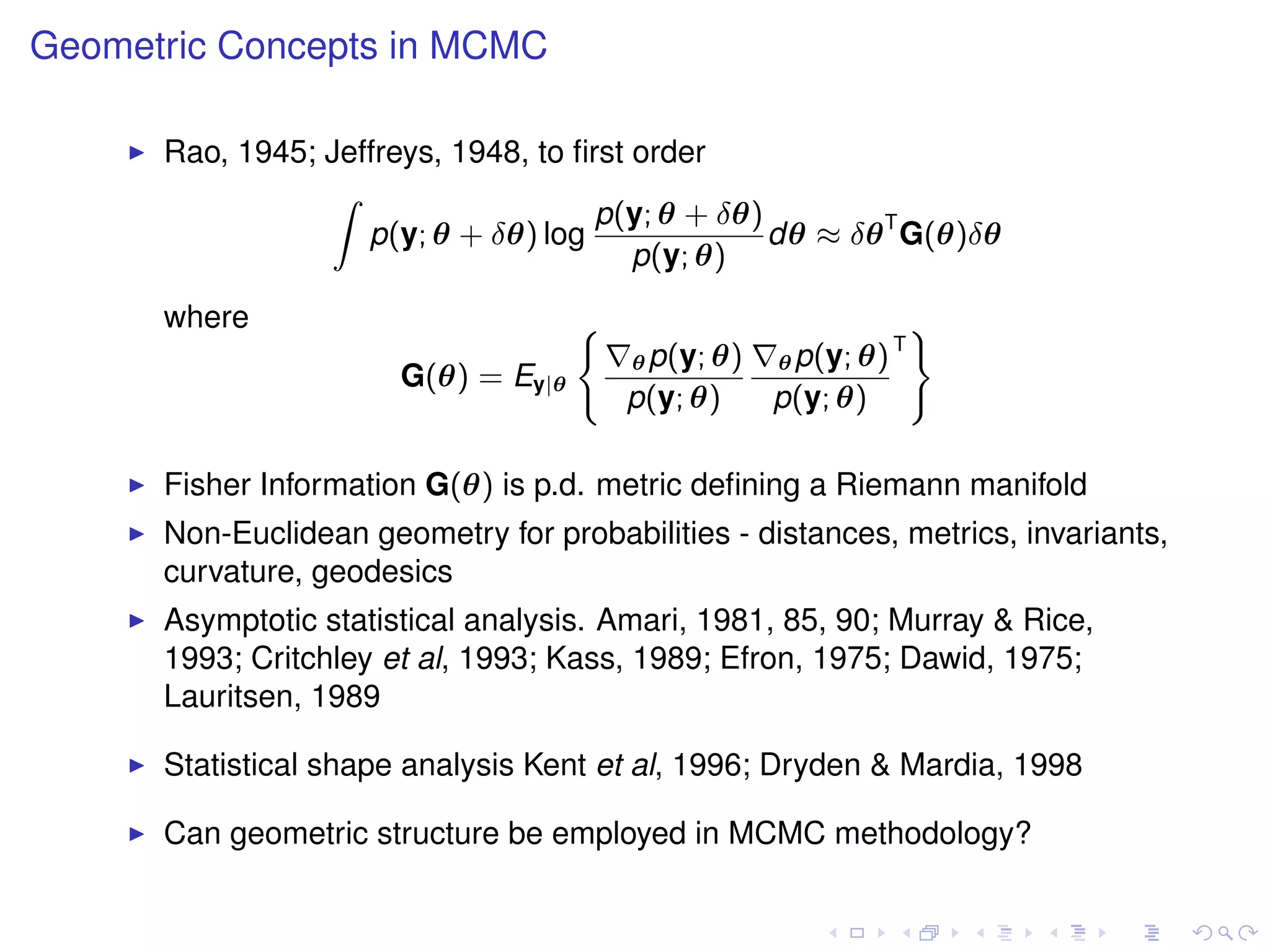
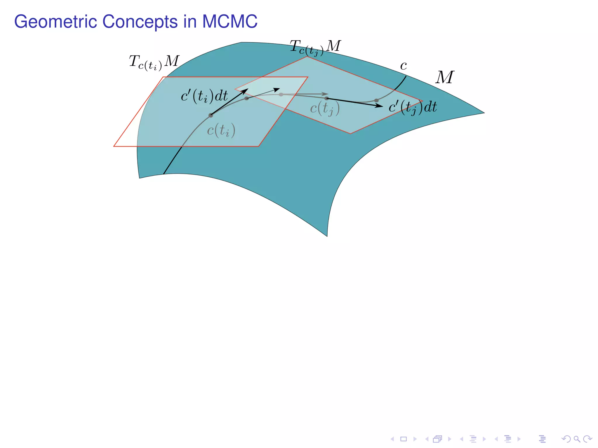
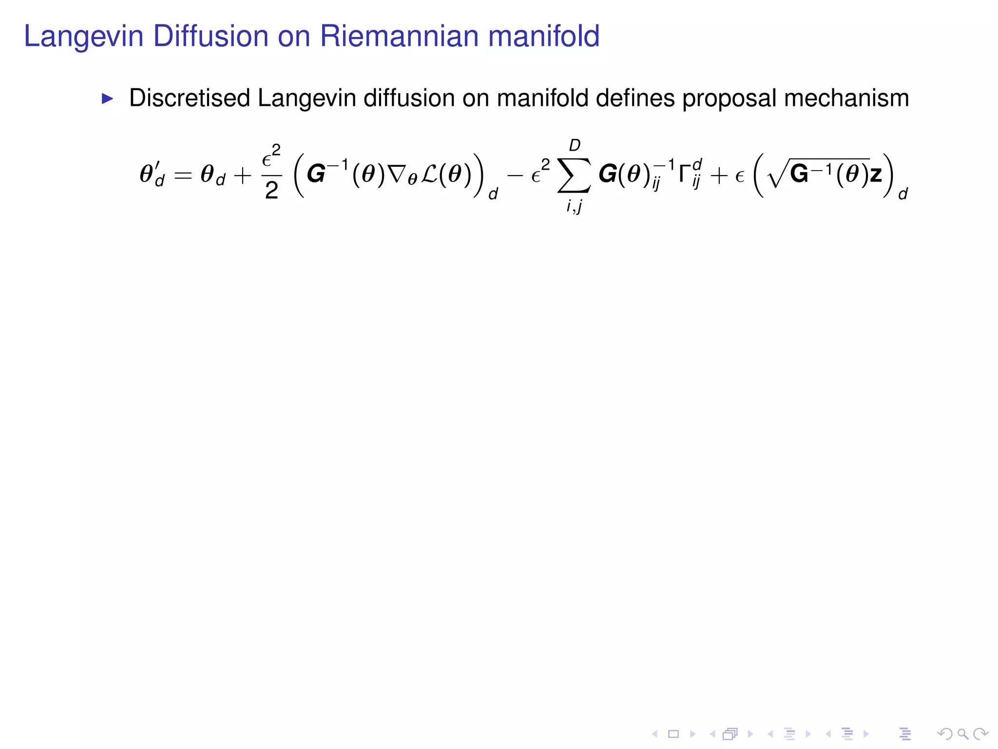
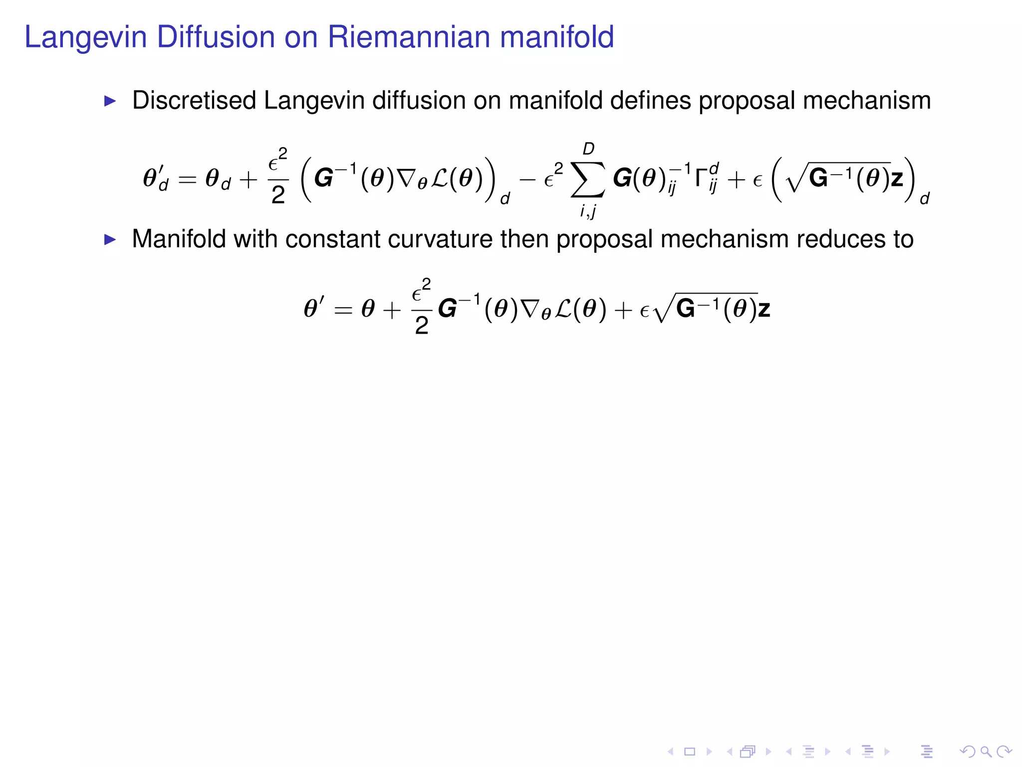
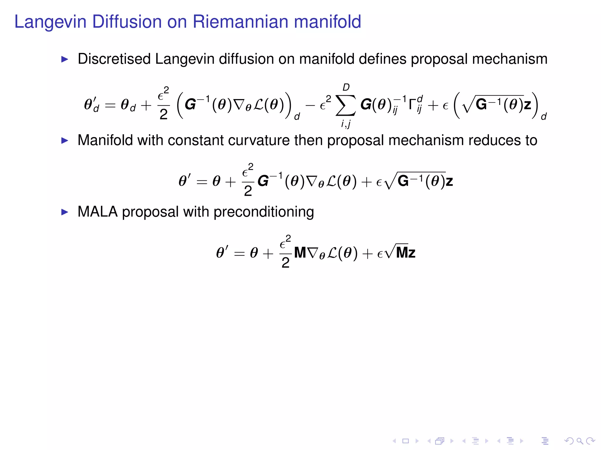
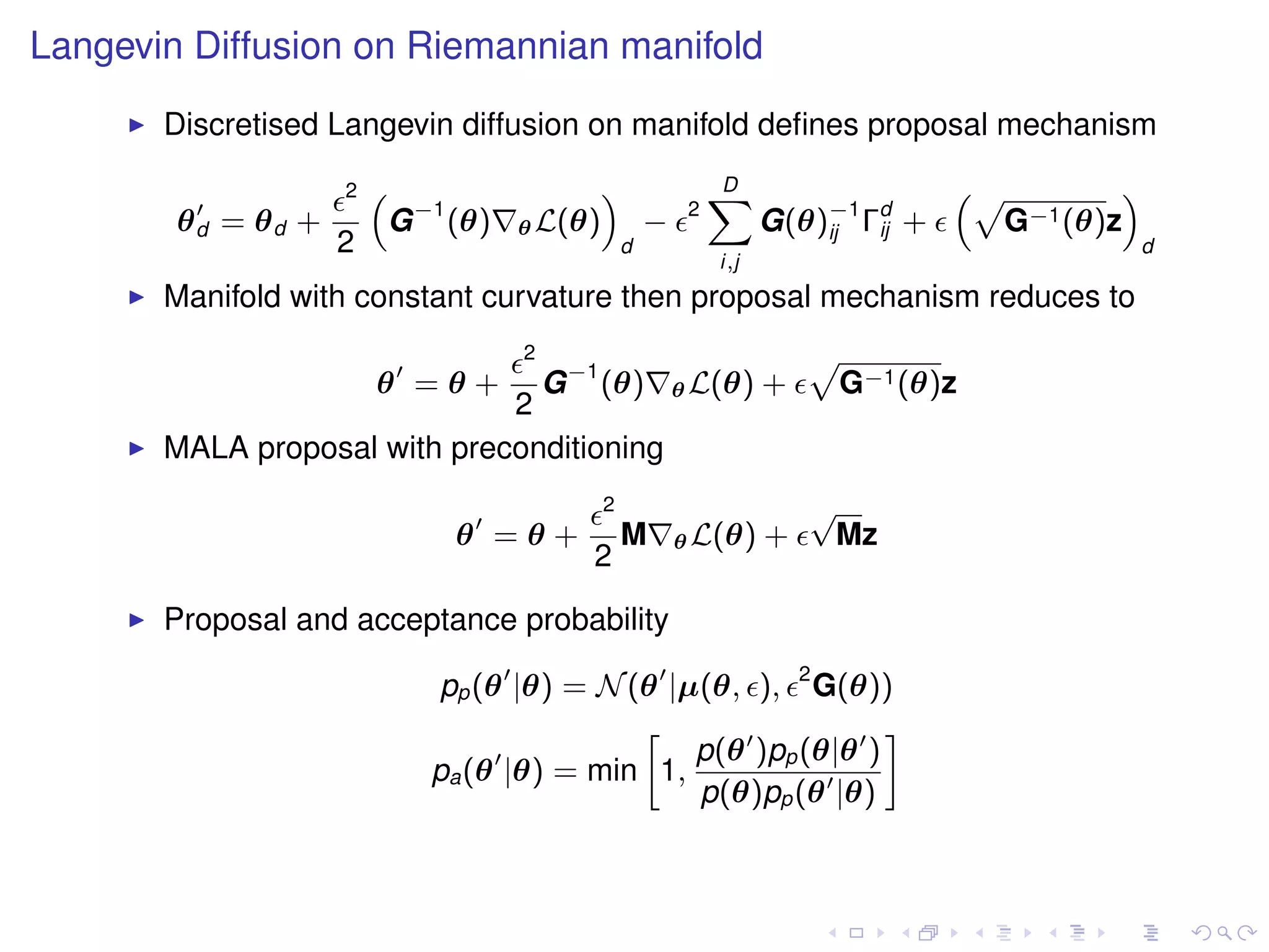
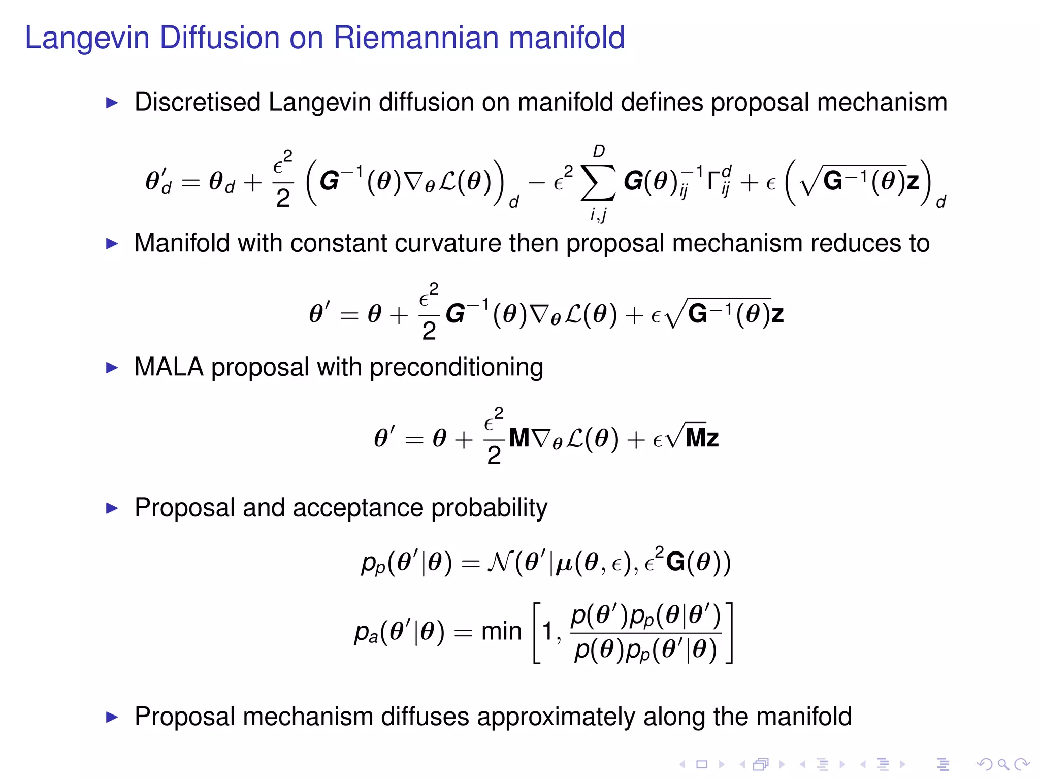
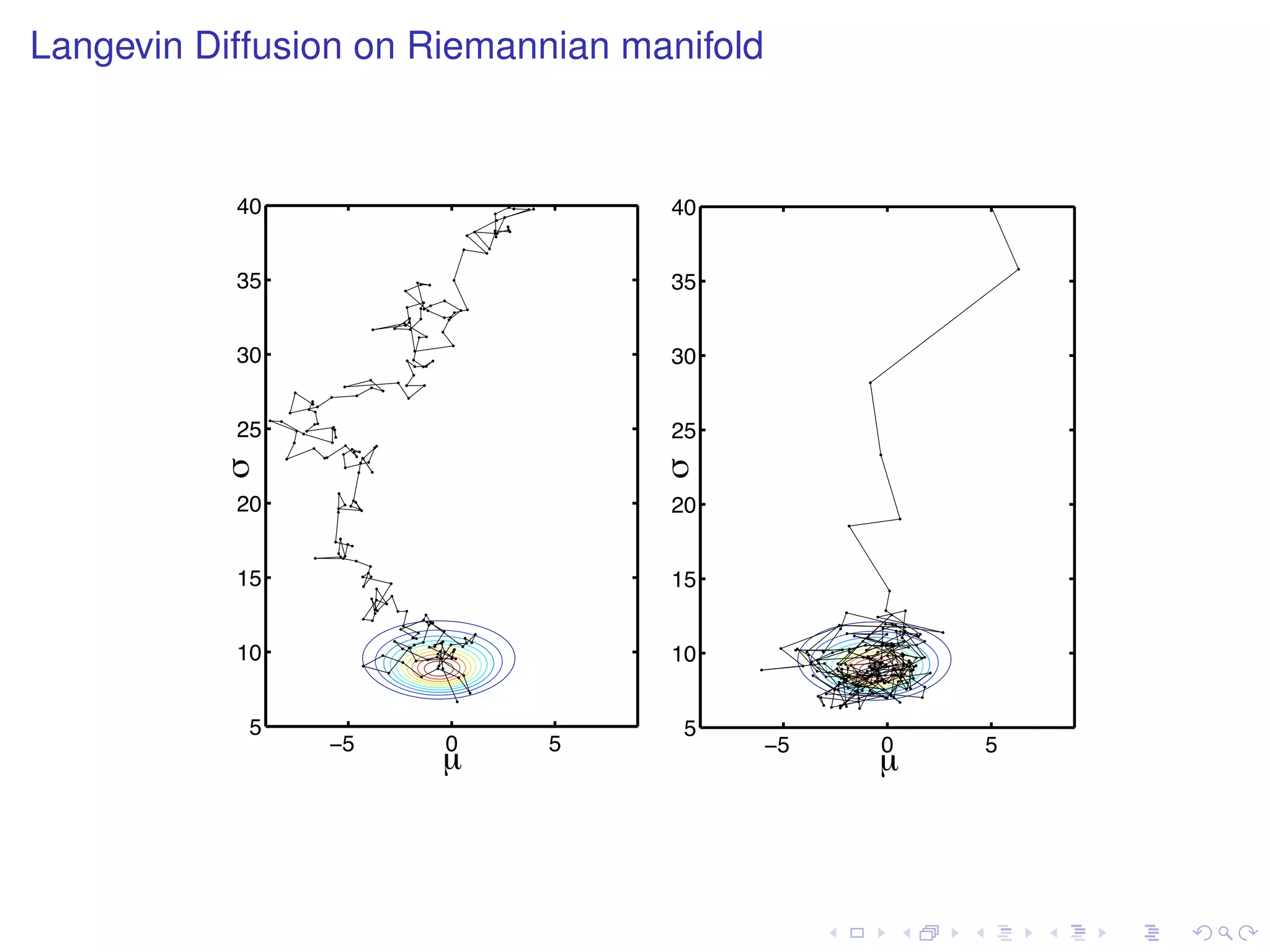
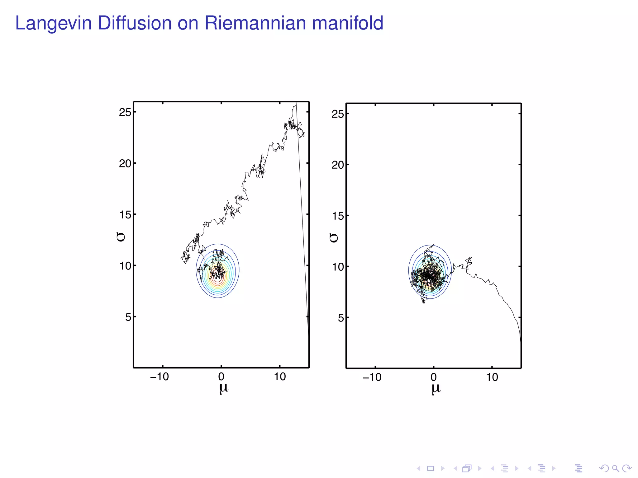
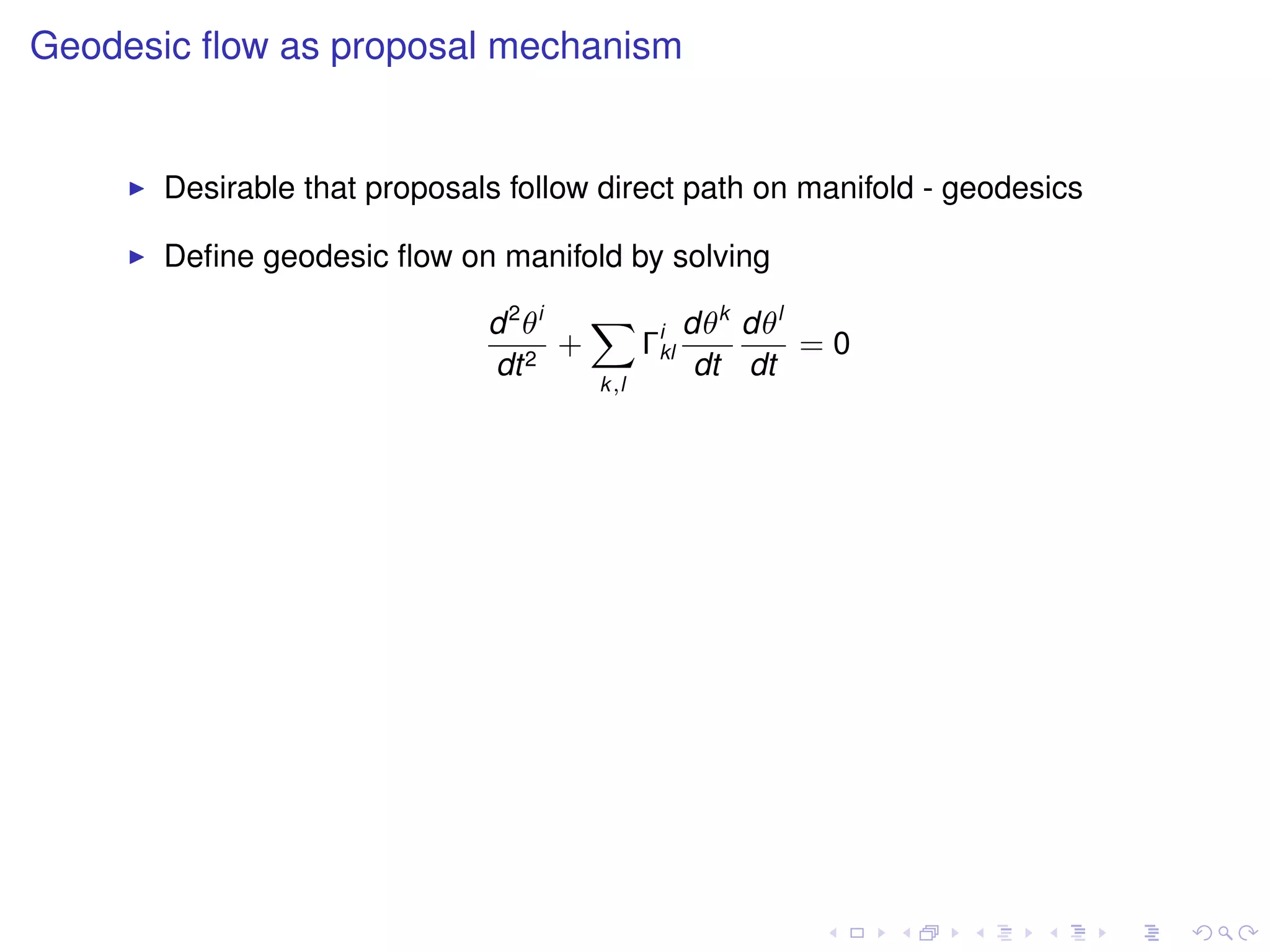
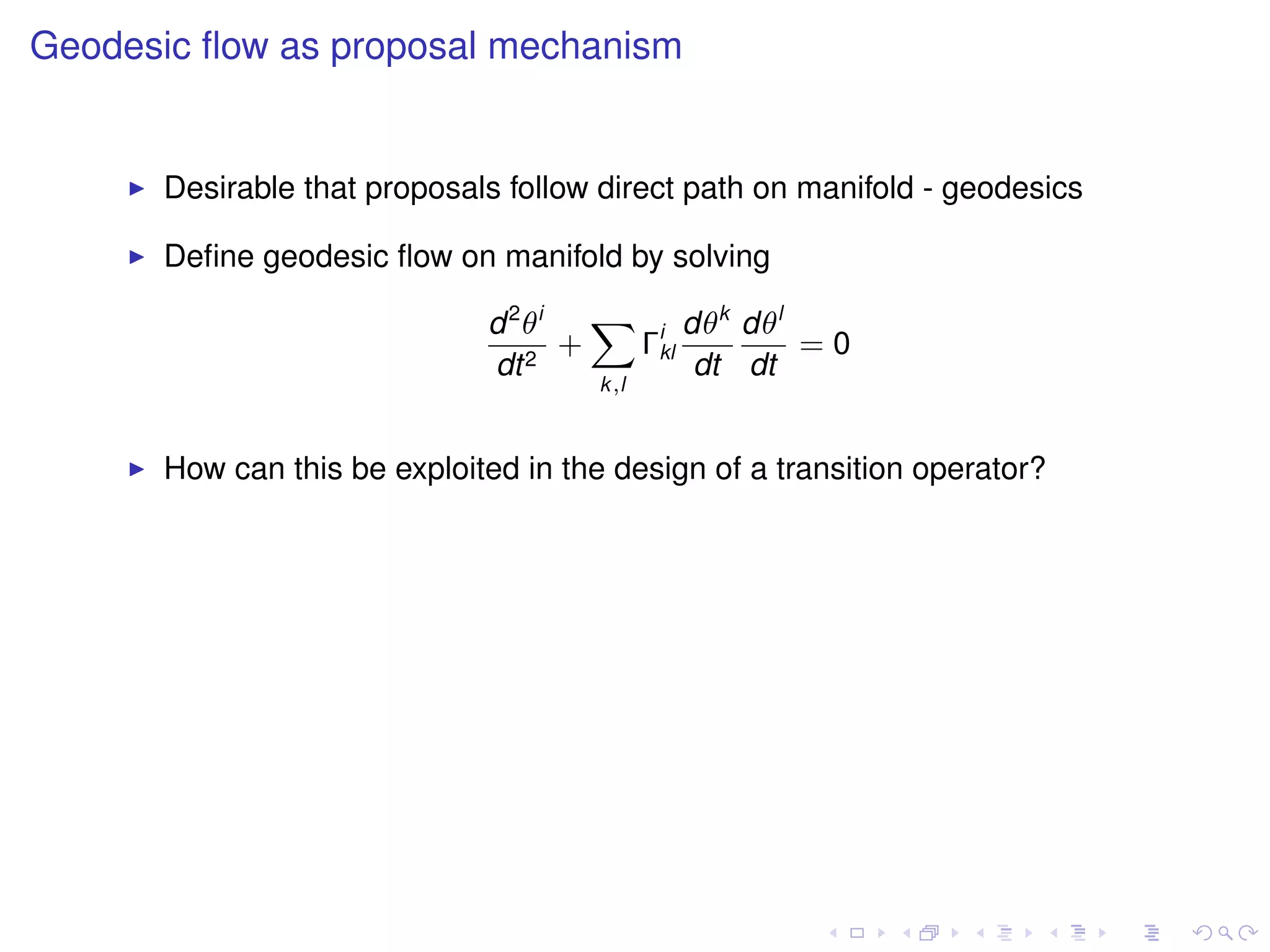
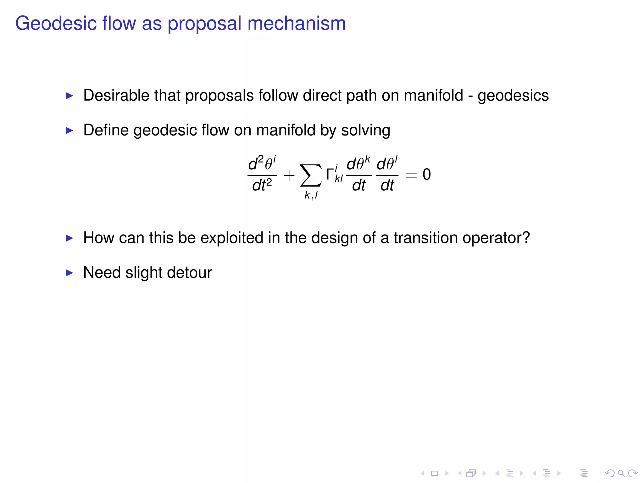
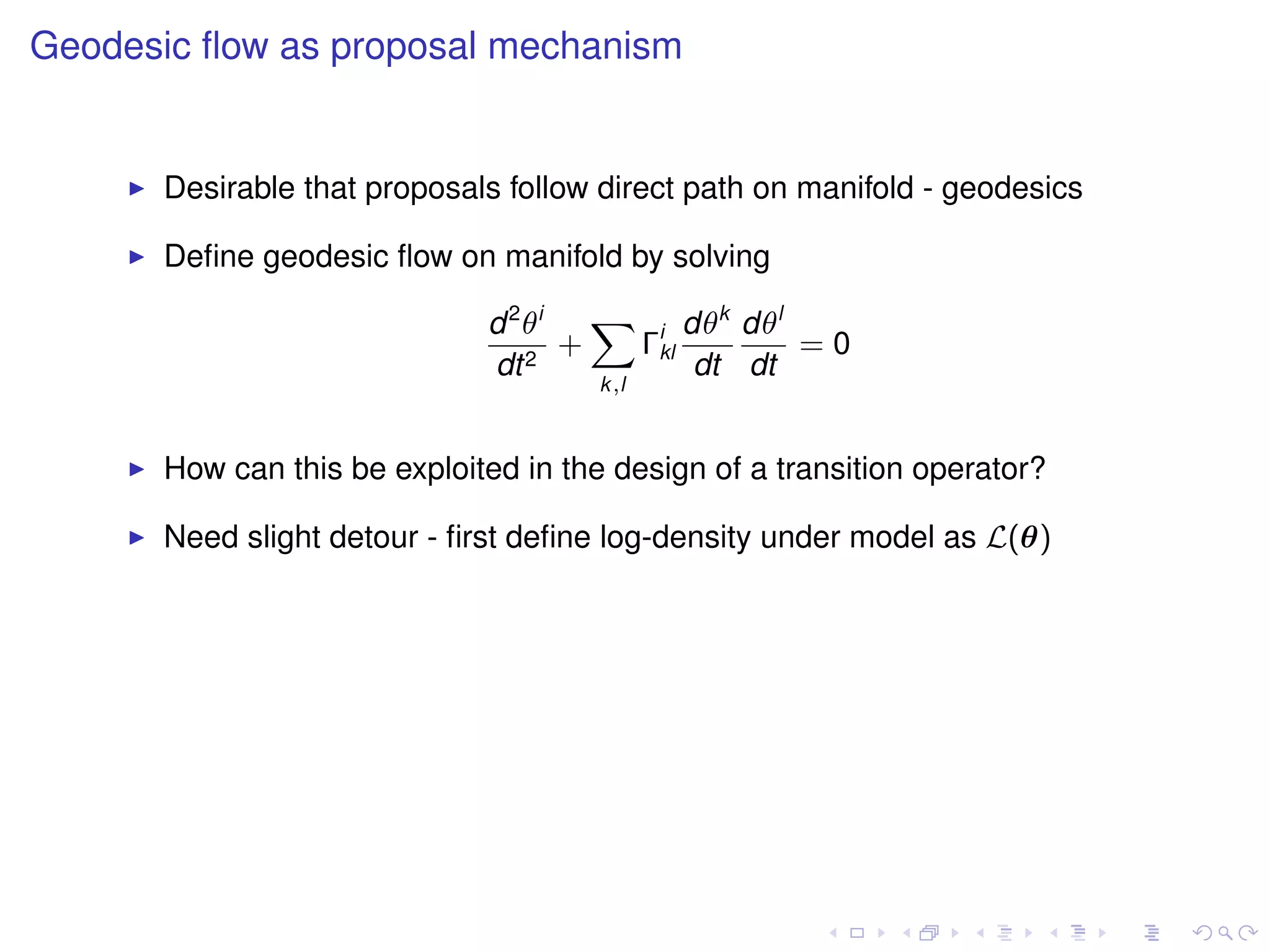
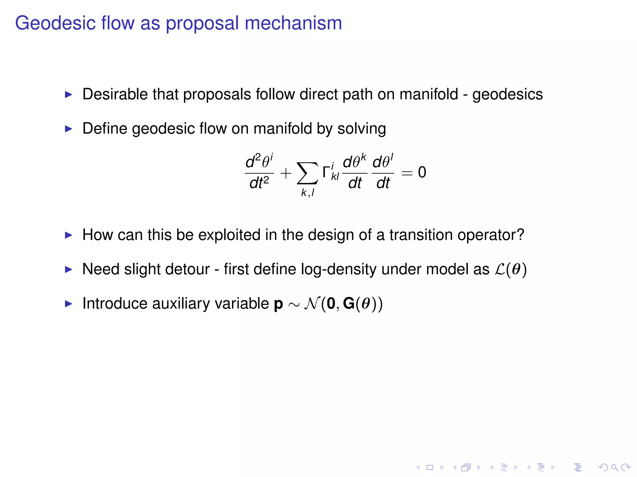
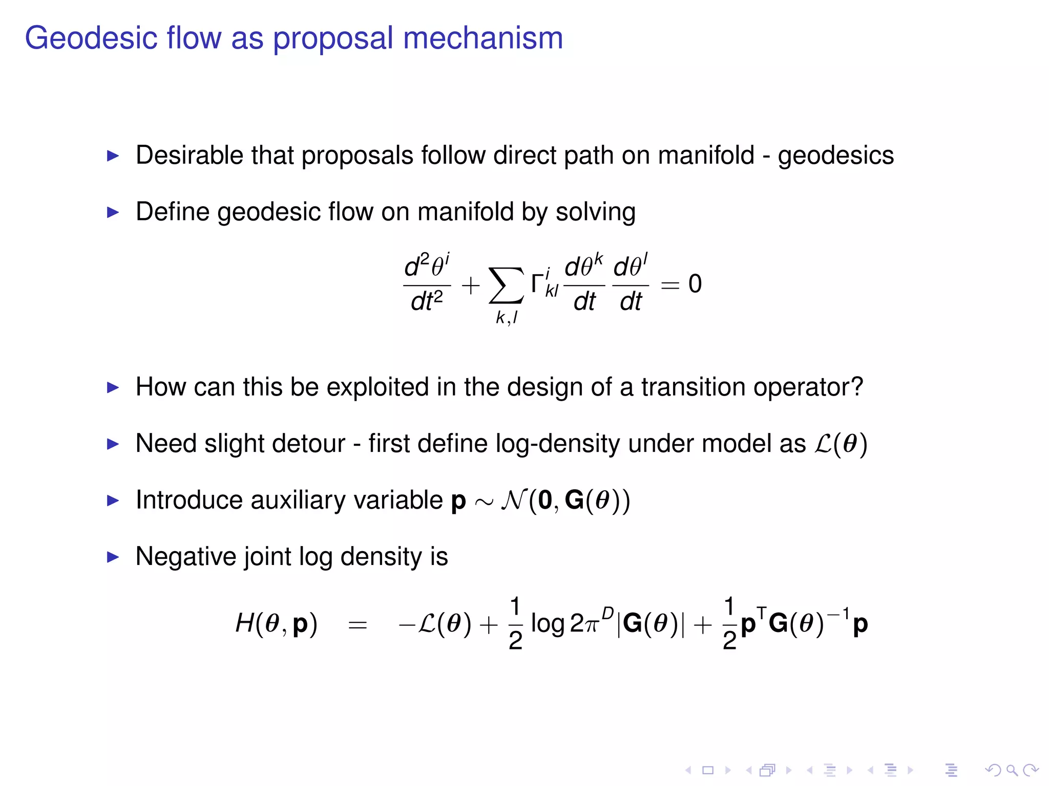
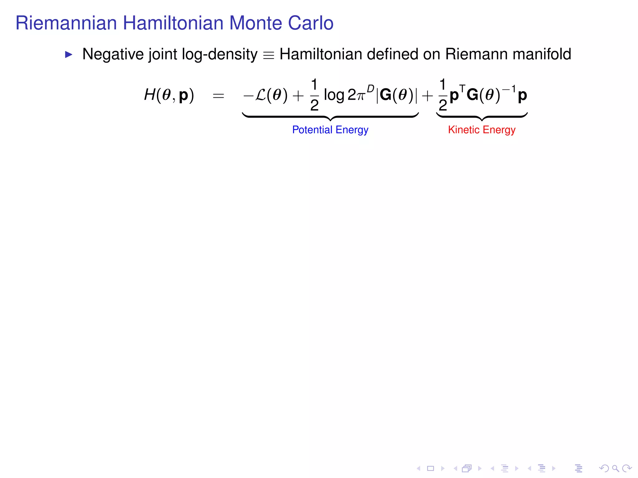
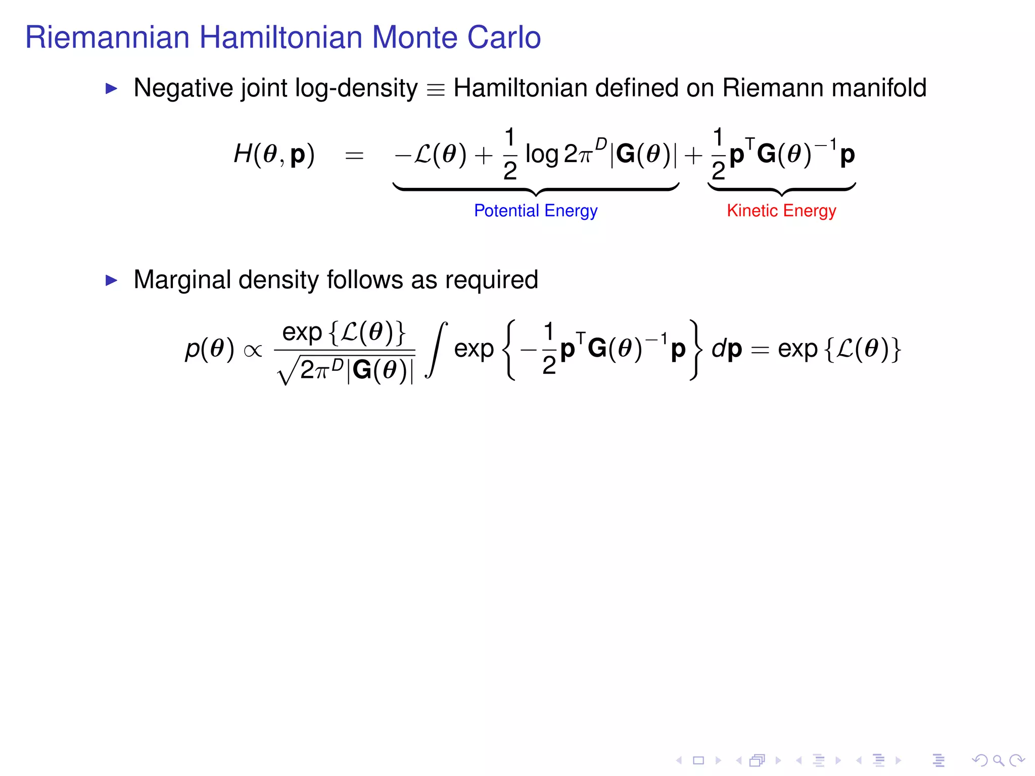
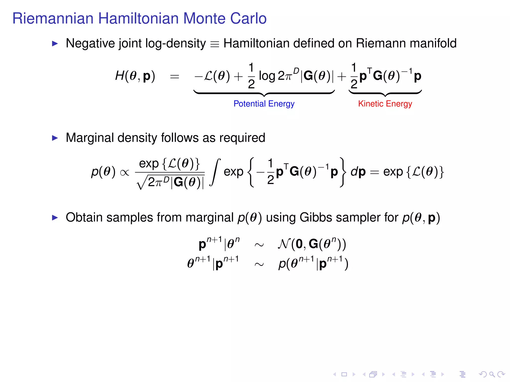
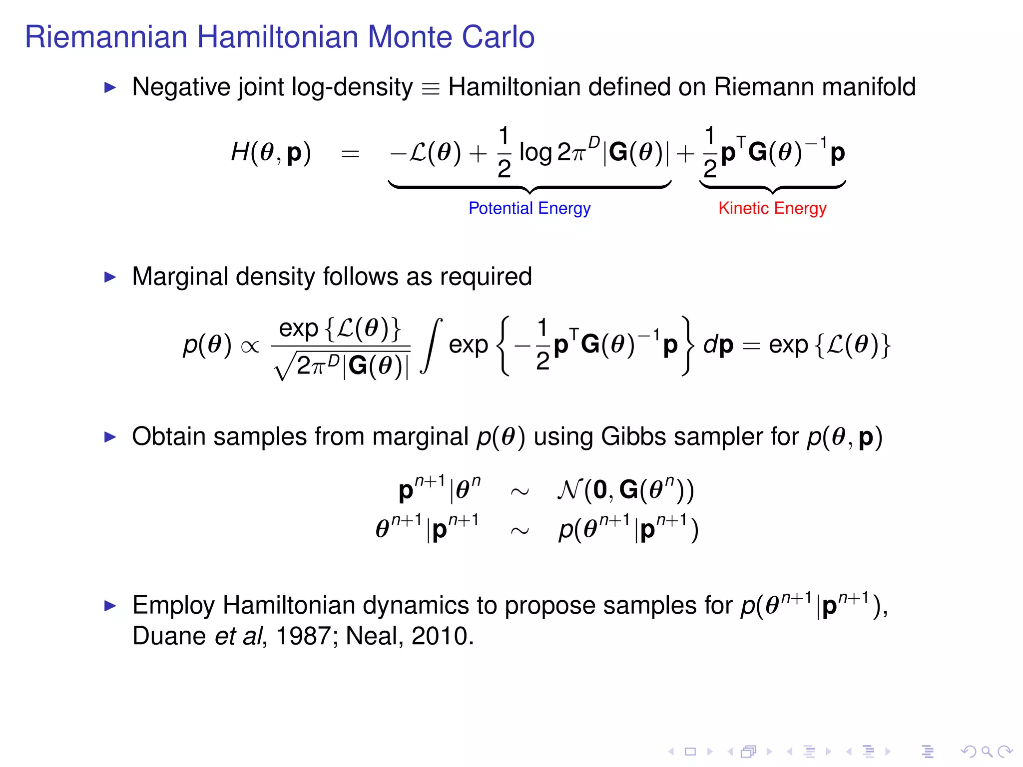
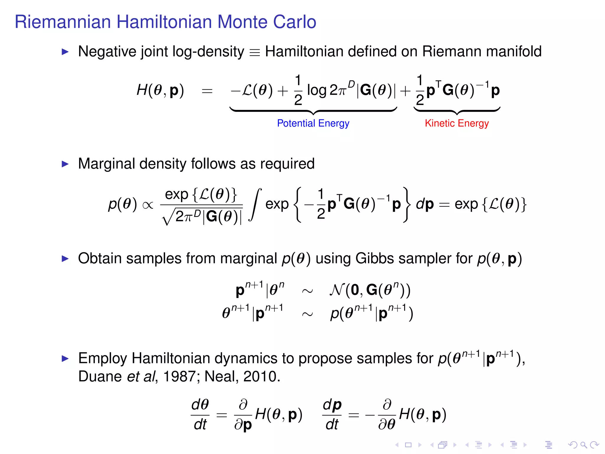
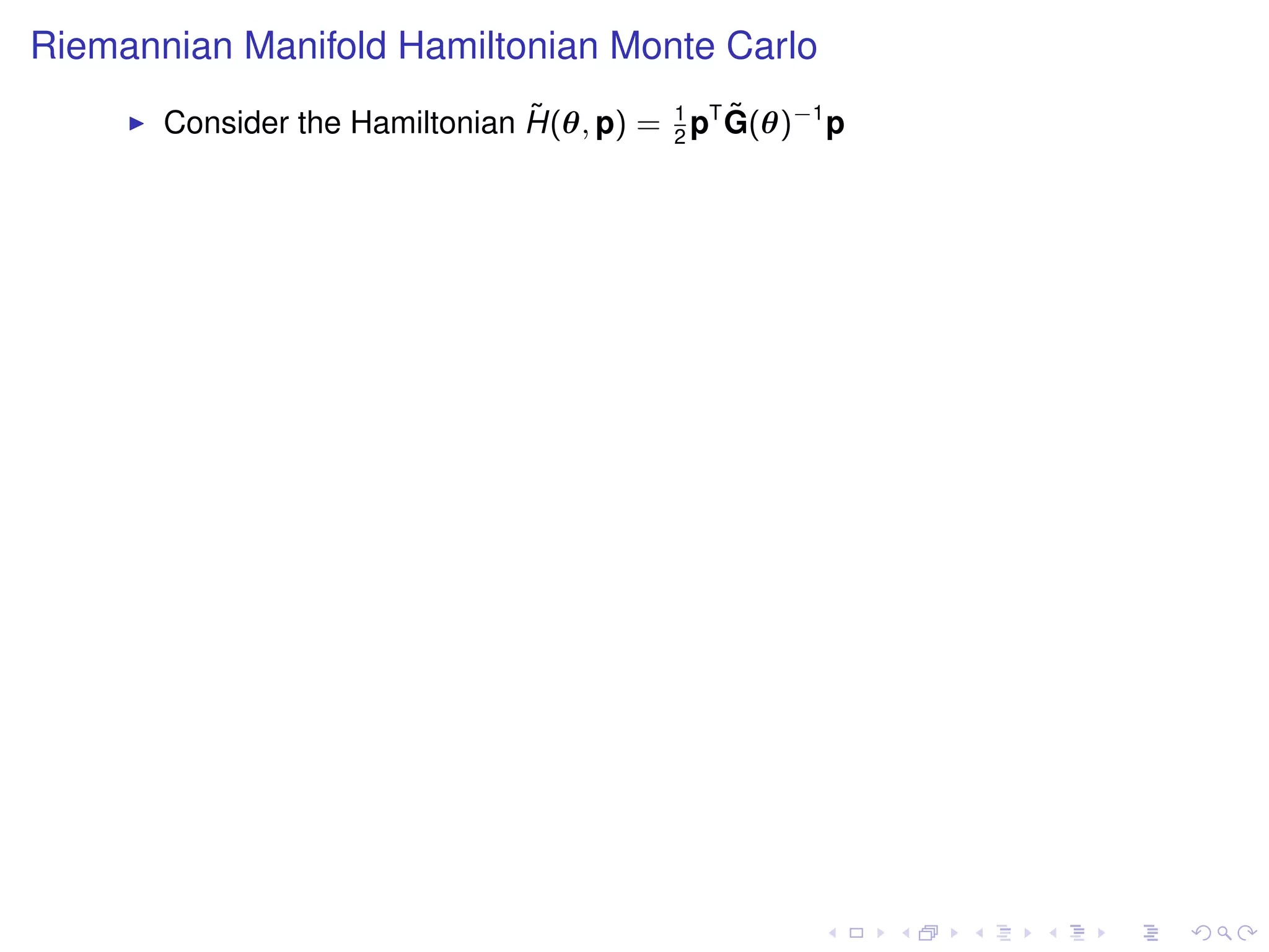
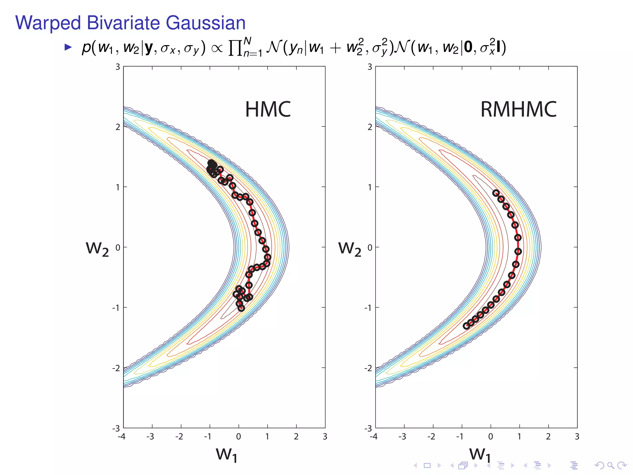
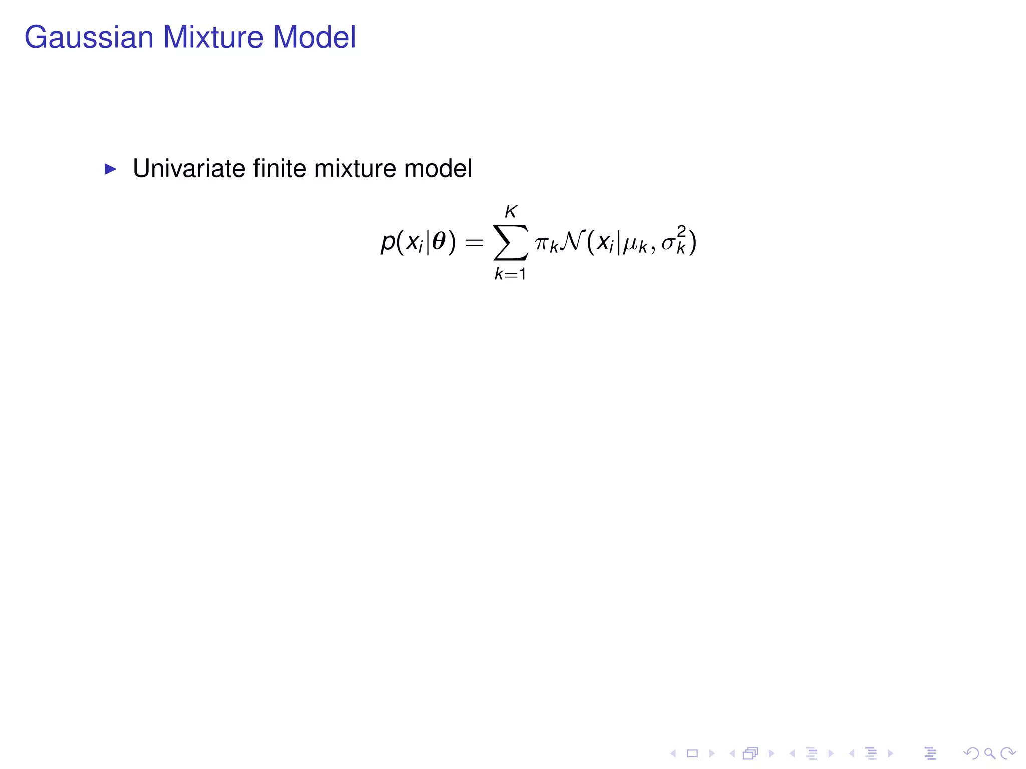
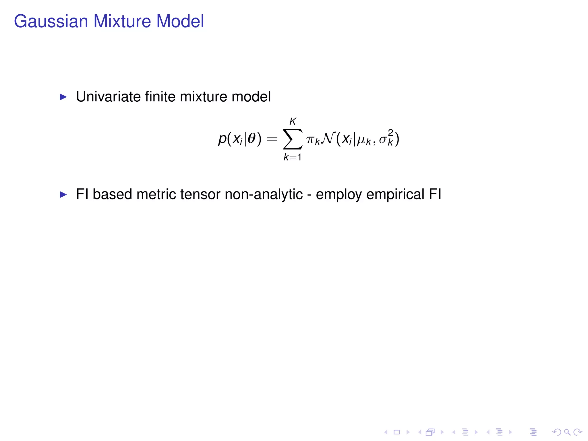
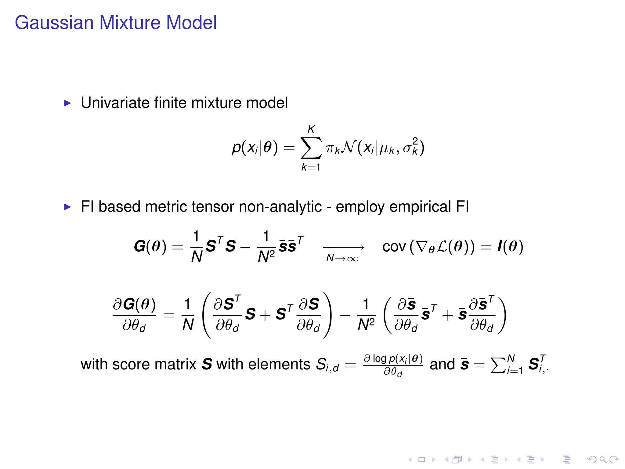
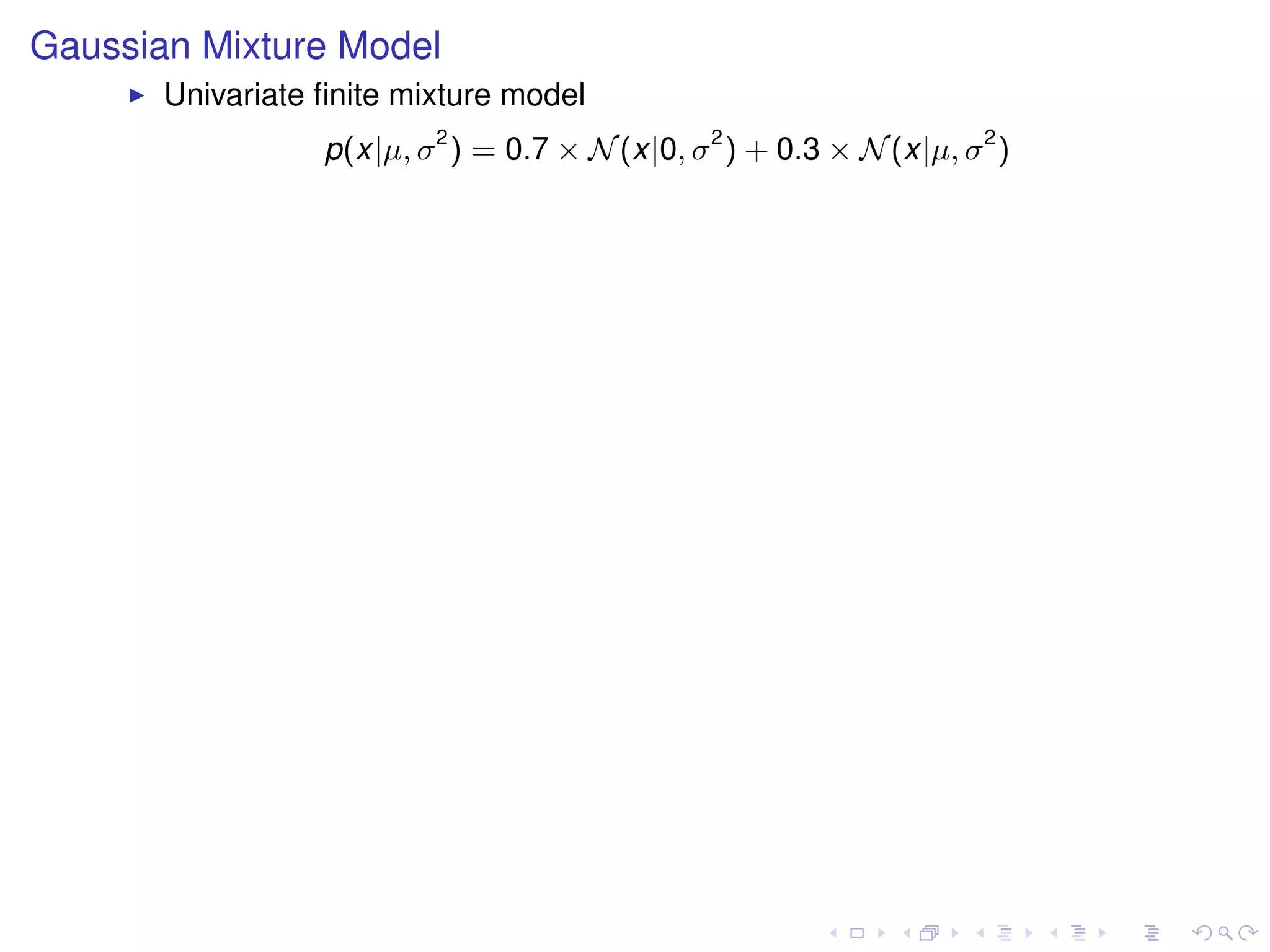
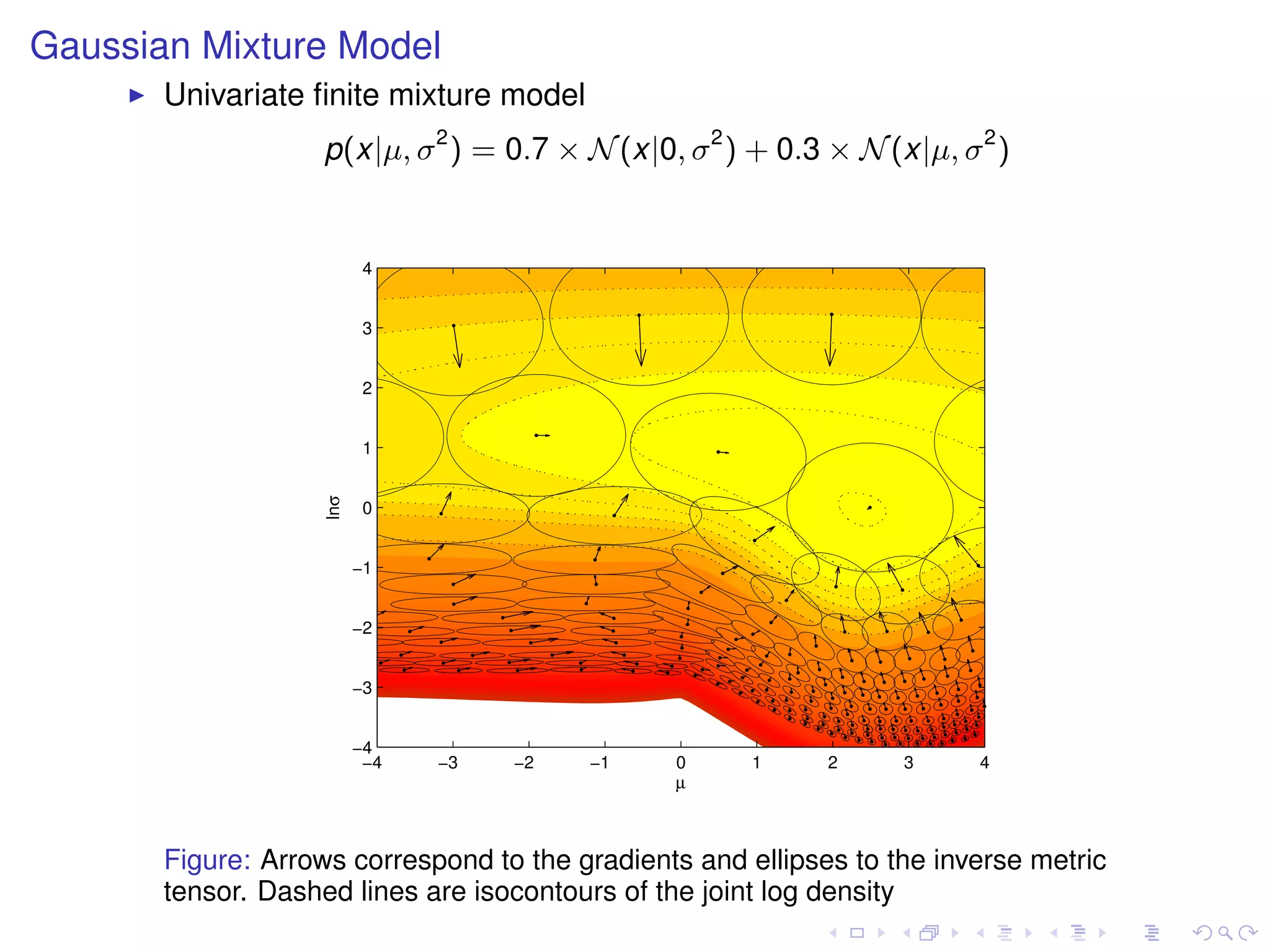
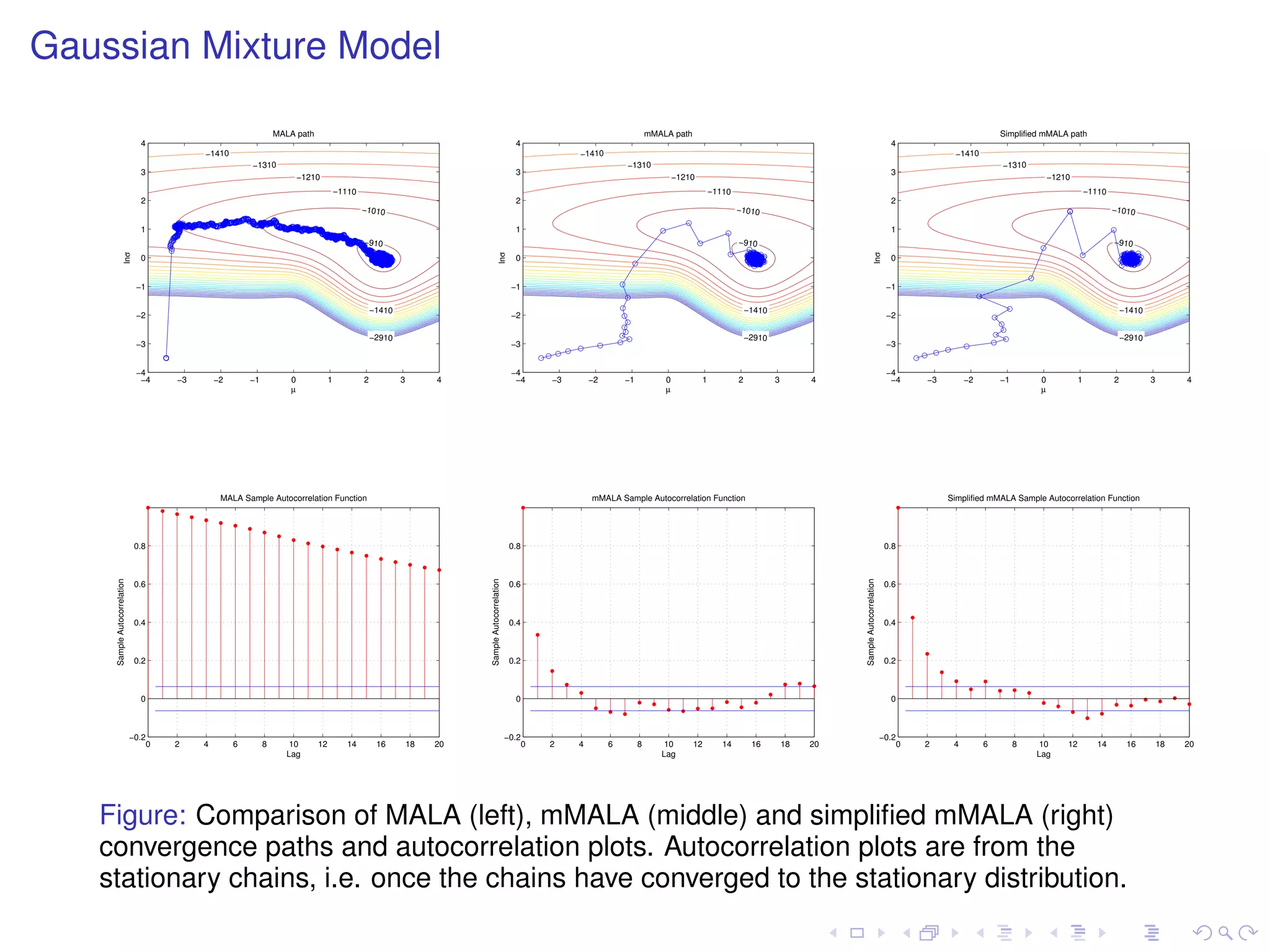
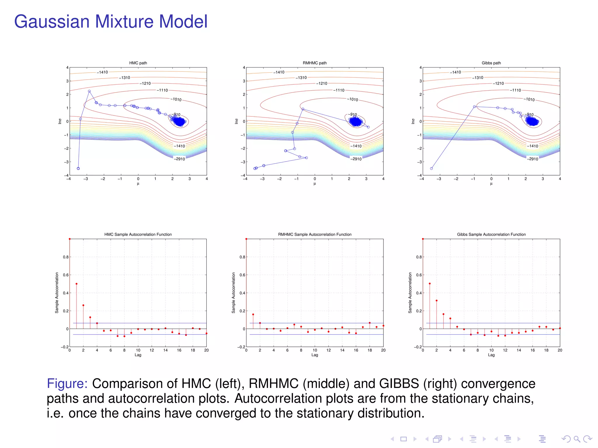
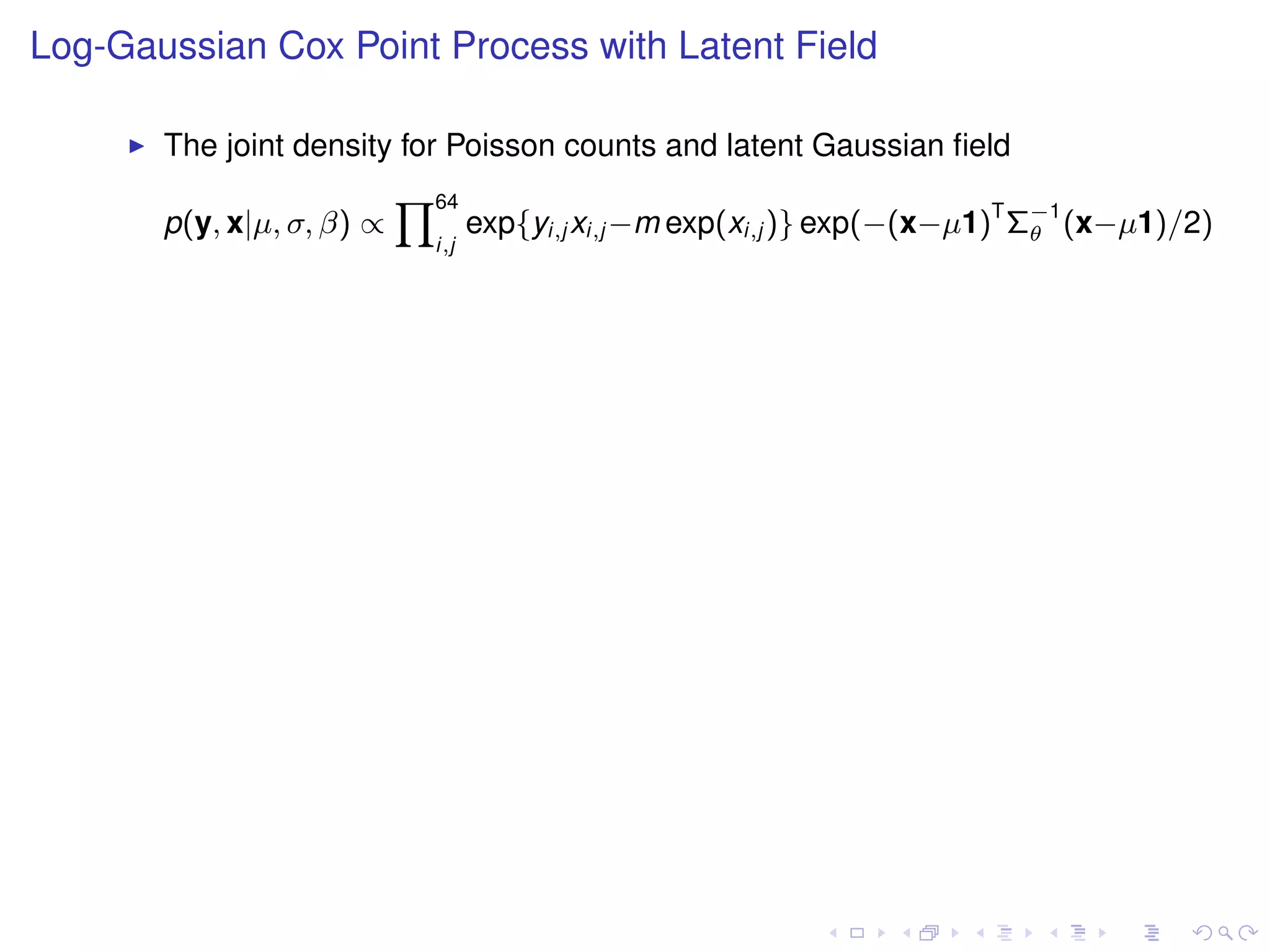
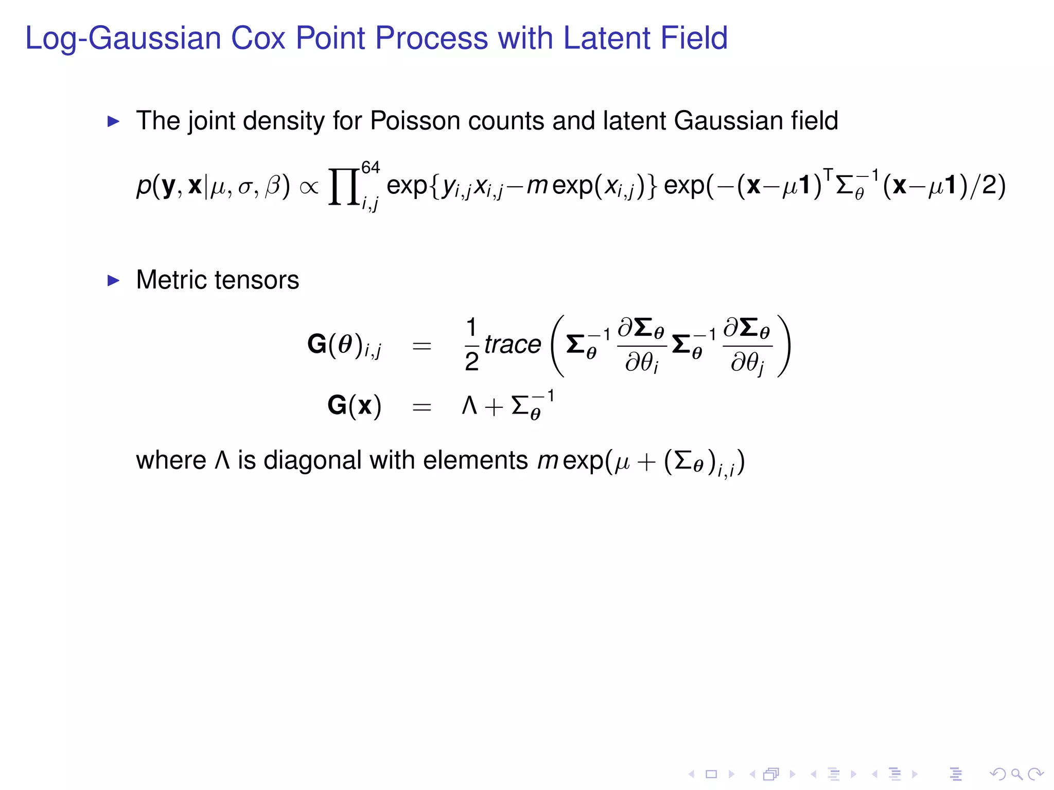
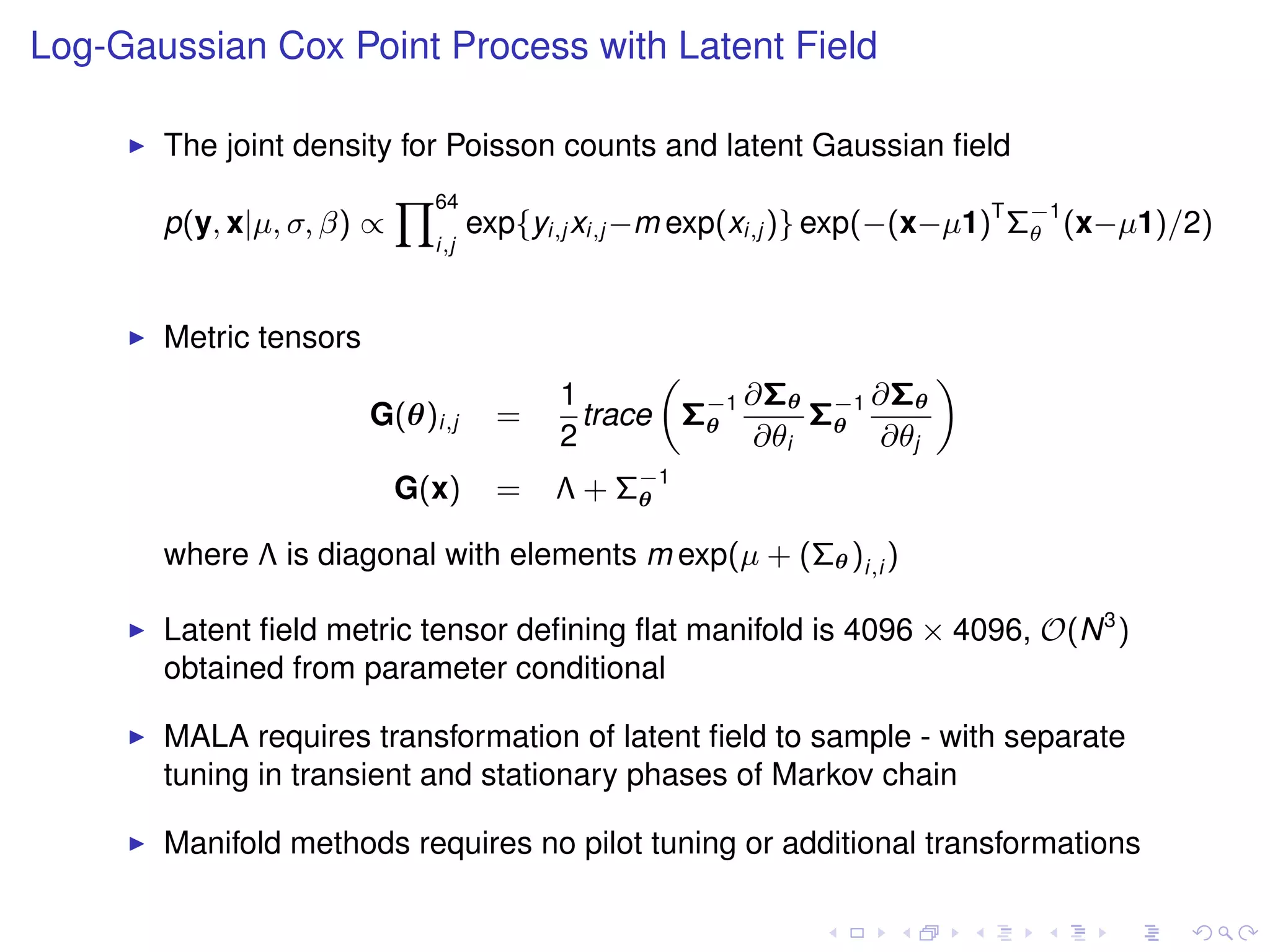
Manifold Monte Carlo Methods

            Mark Girolami

      Department of Statistical Science
         University College London

      Joint work with Ben Calderhead


Research Section Ordinary Meeting

   The Royal Statistical Society
        October 13, 2010
Riemann manifold Langevin and Hamiltonian Monte Carlo Methods


Riemann manifold Langevin and Hamiltonian Monte Carlo Methods


       Riemann manifold Langevin and Hamiltonian Monte Carlo Methods
       Girolami, M. & Calderhead, B., J.R.Statist. Soc. B (2011), 73, 2, 1 - 37.
Riemann manifold Langevin and Hamiltonian Monte Carlo Methods


       Riemann manifold Langevin and Hamiltonian Monte Carlo Methods
       Girolami, M. & Calderhead, B., J.R.Statist. Soc. B (2011), 73, 2, 1 - 37.

       Advanced Monte Carlo methodology founded on geometric principles
Talk Outline


        Motivation to improve MCMC capability for challenging problems
Talk Outline


        Motivation to improve MCMC capability for challenging problems

        Stochastic diffusion as adaptive proposal process
Talk Outline


        Motivation to improve MCMC capability for challenging problems

        Stochastic diffusion as adaptive proposal process

        Exploring geometric concepts in MCMC methodology
Talk Outline


        Motivation to improve MCMC capability for challenging problems

        Stochastic diffusion as adaptive proposal process

        Exploring geometric concepts in MCMC methodology

        Diffusions across Riemann manifold as proposal mechanism
Talk Outline


        Motivation to improve MCMC capability for challenging problems

        Stochastic diffusion as adaptive proposal process

        Exploring geometric concepts in MCMC methodology

        Diffusions across Riemann manifold as proposal mechanism

        Deterministic geodesic flows on manifold form basis of MCMC methods
        Illustrative Examples:-
            Warped Bivariate Gaussian
            Gaussian mixture model
            Log-Gaussian Cox process


        Conclusions
Motivation Simulation Based Inference


       Monte Carlo method employs samples from p(θ) to obtain estimate
                    Z
                                     1 X                    1
                       φ(θ)p(θ)dθ =         φ(θ n ) + O(N − 2 )
                                    N     n


       Draw θ n from ergodic Markov process with stationary distribution p(θ)
       Construct process in two parts
           Propose a move θ → θ with probability pp (θ |θ)
           accept or reject proposal with probability
                                               »                    –
                                                     p(θ )pp (θ|θ )
                                pa (θ |θ) = min 1,
                                                      p(θ)pp (θ |θ)

       Efficiency dependent on pp (θ |θ) defining proposal mechanism

       Success of MCMC reliant upon appropriate proposal design
Adaptive Proposal Distributions - Exploit Discretised Diffusion

        For θ ∈ RD with density p(θ), L(θ) ≡ log p(θ), define Langevin diffusion
                                      1
                            dθ(t) =       θ L(θ(t))dt   + db(t)
                                      2
Adaptive Proposal Distributions - Exploit Discretised Diffusion

        For θ ∈ RD with density p(θ), L(θ) ≡ log p(θ), define Langevin diffusion
                                      1
                            dθ(t) =       θ L(θ(t))dt   + db(t)
                                      2
        First order Euler-Maruyama discrete integration of diffusion
                                             2
                        θ(τ + ) = θ(τ ) +        θ L(θ(τ ))   + z(τ )
                                            2
Adaptive Proposal Distributions - Exploit Discretised Diffusion

        For θ ∈ RD with density p(θ), L(θ) ≡ log p(θ), define Langevin diffusion
                                      1
                            dθ(t) =           θ L(θ(t))dt   + db(t)
                                      2
        First order Euler-Maruyama discrete integration of diffusion
                                                 2
                        θ(τ + ) = θ(τ ) +            θ L(θ(τ ))   + z(τ )
                                                2
        Proposal                                                            2
                                          2
             pp (θ |θ) = N (θ |µ(θ, ),        I) with µ(θ, ) = θ +              θ L(θ)
                                                                            2
Adaptive Proposal Distributions - Exploit Discretised Diffusion

        For θ ∈ RD with density p(θ), L(θ) ≡ log p(θ), define Langevin diffusion
                                       1
                             dθ(t) =           θ L(θ(t))dt   + db(t)
                                       2
        First order Euler-Maruyama discrete integration of diffusion
                                                  2
                         θ(τ + ) = θ(τ ) +            θ L(θ(τ ))   + z(τ )
                                                 2
        Proposal                                                             2
                                           2
             pp (θ |θ) = N (θ |µ(θ, ),         I) with µ(θ, ) = θ +              θ L(θ)
                                                                             2
        Acceptance probability to correct for bias
                                           »                   –
                                                p(θ )pp (θ|θ )
                         pa (θ |θ) = min 1,
                                                p(θ)pp (θ |θ)
        Isotropic diffusion inefficient, employ pre-conditioning
                                                          √
                              θ = θ + 2 M θ L(θ)/2 +        Mz

        How to set M systematically? Tuning in transient & stationary phases
Geometric Concepts in MCMC

      Rao, 1945; Jeffreys, 1948, to first order
                 Z
                                      p(y; θ + δθ)
                    p(y; θ + δθ) log               dθ ≈ δθ T G(θ)δθ
                                         p(y; θ)
Geometric Concepts in MCMC

      Rao, 1945; Jeffreys, 1948, to first order
                 Z
                                      p(y; θ + δθ)
                    p(y; θ + δθ) log               dθ ≈ δθ T G(θ)δθ
                                         p(y; θ)
      where                          (                               )
                                                                 T
                                         θ p(y; θ)   θ p(y; θ)
                       G(θ) = Ey|θ
                                         p(y; θ)     p(y; θ)

      Fisher Information G(θ) is p.d. metric defining a Riemann manifold
      Non-Euclidean geometry for probabilities - distances, metrics, invariants,
      curvature, geodesics
      Asymptotic statistical analysis. Amari, 1981, 85, 90; Murray & Rice,
      1993; Critchley et al, 1993; Kass, 1989; Efron, 1975; Dawid, 1975;
      Lauritsen, 1989

      Statistical shape analysis Kent et al, 1996; Dryden & Mardia, 1998

      Can geometric structure be employed in MCMC methodology?
Geometric Concepts in MCMC


      Tangent space - local metric defined by δθ T G(θ)δθ =
                                                             P
                                                             k ,l   gkl δθk δθl
Geometric Concepts in MCMC


      Tangent space - local metric defined by δθ T G(θ)δθ = k ,l gkl δθk δθl
                                                            P

      Christoffel symbols - characterise connection on curved manifold
Geometric Concepts in MCMC


      Tangent space - local metric defined by δθ T G(θ)δθ = k ,l gkl δθk δθl
                                                             P

      Christoffel symbols - characterise connection on curved manifold
                                       „                     «
                             1 X im ∂gmk        ∂gml    ∂gkl
                      Γikl =       g          +      − m
                             2 m          ∂θl    ∂θk    ∂θ

      Geodesics - shortest path between two points on manifold
                              d 2 θi   X i dθk dθl
                                     +  Γkl        =0
                              dt 2          dt dt
                                      k,l
Illustration of Geometric Concepts


       Consider Normal density p(x|µ, σ) = Nx (µ, σ)
Illustration of Geometric Concepts


       Consider Normal density p(x|µ, σ) = Nx (µ, σ)

       Local inner product on tangent space defined by metric tensor, i.e.
       δθ T G(θ)δθ, where θ = (µ, σ)T
Illustration of Geometric Concepts


       Consider Normal density p(x|µ, σ) = Nx (µ, σ)

       Local inner product on tangent space defined by metric tensor, i.e.
       δθ T G(θ)δθ, where θ = (µ, σ)T

       Metric is Fisher Information
                                              σ −2
                                          »                  –
                                                      0
                              G(µ, σ) =
                                               0     2σ −2
Illustration of Geometric Concepts


       Consider Normal density p(x|µ, σ) = Nx (µ, σ)

       Local inner product on tangent space defined by metric tensor, i.e.
       δθ T G(θ)δθ, where θ = (µ, σ)T

       Metric is Fisher Information
                                               σ −2
                                           »                  –
                                                       0
                               G(µ, σ) =
                                                0     2σ −2


       Inner-product σ −2 (δµ2 + 2δσ 2 ) so densities N (0, 1) & N (1, 1) further
       apart than the densities N (0, 2) & N (1, 2) - distance non-Euclidean

       Metric tensor for univariate Normal defines a Hyperbolic Space
M.C. Escher, Heaven and Hell, 1960
Langevin Diffusion on Riemannian manifold
       Discretised Langevin diffusion on manifold defines proposal mechanism
                    2   “                    ”               D
                                                             X                   “p        ”
        θd = θd +        G −1 (θ)   θ L(θ)           −   2
                                                                   G(θ)−1 Γd +
                                                                       ij  ij      G−1 (θ)z
                    2                            d                                             d
                                                             i,j
Langevin Diffusion on Riemannian manifold
       Discretised Langevin diffusion on manifold defines proposal mechanism
                    2   “                    ”                D
                                                              X                    “p        ”
        θd = θd +        G −1 (θ)   θ L(θ)           −    2
                                                                    G(θ)−1 Γd +
                                                                        ij  ij       G−1 (θ)z
                    2                            d                                               d
                                                              i,j
       Manifold with constant curvature then proposal mechanism reduces to
                                    2
                                        G −1 (θ)
                                                                        p
                        θ =θ+                            θ L(θ)     +       G−1 (θ)z
                                    2
Langevin Diffusion on Riemannian manifold
       Discretised Langevin diffusion on manifold defines proposal mechanism
                    2   “                    ”                D
                                                              X                    “p        ”
        θd = θd +        G −1 (θ)   θ L(θ)           −    2
                                                                    G(θ)−1 Γd +
                                                                        ij  ij       G−1 (θ)z
                    2                            d                                               d
                                                              i,j
       Manifold with constant curvature then proposal mechanism reduces to
                                    2
                                G −1 (θ) θ L(θ) +
                                                                        p
                        θ =θ+                                               G−1 (θ)z
                              2
       MALA proposal with preconditioning
                                             2                          √
                              θ =θ+              M       θ L(θ)     +    Mz
                                         2

       Proposal and acceptance probability

                            pp (θ |θ) = N (θ |µ(θ, ), 2 G(θ))
                                           »                  –
                                               p(θ )pp (θ|θ )
                            pa (θ |θ) = min 1,
                                               p(θ)pp (θ |θ)

       Proposal mechanism diffuses approximately along the manifold
Langevin Diffusion on Riemannian manifold


           40                      40


           35                      35


           30                      30


           25                      25
          !


                                   !
           20                      20


           15                      15


           10                      10


            5                       5
                −5     0    5               −5   0   5
                       µ                         µ
Langevin Diffusion on Riemannian manifold


           25                      25


           20                      20


           15                      15
          !


                                  !
           10                      10


            5                       5


                −10   0     10          −10   0   10
                      µ                       µ
Geodesic flow as proposal mechanism


      Desirable that proposals follow direct path on manifold - geodesics
Geodesic flow as proposal mechanism


      Desirable that proposals follow direct path on manifold - geodesics

      Define geodesic flow on manifold by solving

                             d 2 θi   X i dθk dθl
                                    +  Γkl        =0
                             dt 2          dt dt
                                     k,l
Geodesic flow as proposal mechanism


      Desirable that proposals follow direct path on manifold - geodesics

      Define geodesic flow on manifold by solving

                             d 2 θi   X i dθk dθl
                                    +  Γkl        =0
                             dt 2          dt dt
                                      k,l


      How can this be exploited in the design of a transition operator?

      Need slight detour
Geodesic flow as proposal mechanism


      Desirable that proposals follow direct path on manifold - geodesics

      Define geodesic flow on manifold by solving

                             d 2 θi   X i dθk dθl
                                    +  Γkl        =0
                             dt 2          dt dt
                                      k,l


      How can this be exploited in the design of a transition operator?

      Need slight detour - first define log-density under model as L(θ)

      Introduce auxiliary variable p ∼ N (0, G(θ))
Geodesic flow as proposal mechanism


      Desirable that proposals follow direct path on manifold - geodesics

      Define geodesic flow on manifold by solving

                              d 2 θi   X i dθk dθl
                                     +  Γkl        =0
                              dt 2          dt dt
                                      k,l


      How can this be exploited in the design of a transition operator?

      Need slight detour - first define log-density under model as L(θ)

      Introduce auxiliary variable p ∼ N (0, G(θ))

      Negative joint log density is
                                        1                  1
               H(θ, p)   =    −L(θ) +     log 2π D |G(θ)| + pT G(θ)−1 p
                                        2                  2
Riemannian Hamiltonian Monte Carlo
       Negative joint log-density ≡ Hamiltonian defined on Riemann manifold
                                    1                 1
               H(θ, p)   =   −L(θ) + log 2π D |G(θ)| + pT G(θ)−1 p
                             |      2 {z           } |2    {z    }
                                   Potential Energy      Kinetic Energy


       Marginal density follows as required
                                 Z                  ff
                   exp {L(θ)}               1
          p(θ) ∝ p                  exp − pT G(θ)−1 p dp = exp {L(θ)}
                     2π D |G(θ)|            2
Riemannian Hamiltonian Monte Carlo
       Negative joint log-density ≡ Hamiltonian defined on Riemann manifold
                                    1                 1
               H(θ, p)   =   −L(θ) + log 2π D |G(θ)| + pT G(θ)−1 p
                             |      2 {z           } |2    {z    }
                                             Potential Energy             Kinetic Energy


       Marginal density follows as required
                                 Z                  ff
                   exp {L(θ)}               1
          p(θ) ∝ p                  exp − pT G(θ)−1 p dp = exp {L(θ)}
                     2π D |G(θ)|            2

       Obtain samples from marginal p(θ) using Gibbs sampler for p(θ, p)

                                 pn+1 |θ n        ∼     N (0, G(θ n ))
                                 n+1        n+1
                             θ         |p         ∼     p(θ n+1 |pn+1 )


       Employ Hamiltonian dynamics to propose samples for p(θ n+1 |pn+1 ),
       Duane et al, 1987; Neal, 2010.
Riemannian Hamiltonian Monte Carlo
       Negative joint log-density ≡ Hamiltonian defined on Riemann manifold
                                     1                 1
               H(θ, p)    =   −L(θ) + log 2π D |G(θ)| + pT G(θ)−1 p
                              |      2 {z           } |2    {z    }
                                              Potential Energy             Kinetic Energy


       Marginal density follows as required
                                 Z                  ff
                   exp {L(θ)}               1
          p(θ) ∝ p                  exp − pT G(θ)−1 p dp = exp {L(θ)}
                     2π D |G(θ)|            2

       Obtain samples from marginal p(θ) using Gibbs sampler for p(θ, p)

                                  pn+1 |θ n        ∼     N (0, G(θ n ))
                                  n+1        n+1
                              θ         |p         ∼     p(θ n+1 |pn+1 )


       Employ Hamiltonian dynamics to propose samples for p(θ n+1 |pn+1 ),
       Duane et al, 1987; Neal, 2010.
                         dθ    ∂                       dp     ∂
                            =    H(θ, p)                  = − H(θ, p)
                         dt   ∂p                       dt    ∂θ
Riemannian Manifold Hamiltonian Monte Carlo
                                ˜              ˜
       Consider the Hamiltonian H(θ, p) = 1 pT G(θ)−1 p
                                          2
Riemannian Manifold Hamiltonian Monte Carlo
                                ˜              ˜
       Consider the Hamiltonian H(θ, p) = 1 pT G(θ)−1 p
                                          2

       Hamiltonians with only a quadratic kinetic energy term exactly describe
       geodesic flow on the coordinate space θ with metric G ˜

       However our Hamiltonian is H(θ, p) = V (θ) + 1 pT G(θ)−1 p
                                                    2

                   ˜
       If we define G(θ) = G(θ) × (h − V (θ)), where h is a constant H(θ, p)

       Then the Maupertuis principle tells us that the Hamiltonian flow for
                   ˜
       H(θ, p) and H(θ, p) are equivalent along energy level h

       The solution of
                         dθ    ∂            dp     ∂
                            =    H(θ, p)       = − H(θ, p)
                         dt   ∂p            dt    ∂θ
Riemannian Manifold Hamiltonian Monte Carlo
                                ˜              ˜
       Consider the Hamiltonian H(θ, p) = 1 pT G(θ)−1 p
                                          2

       Hamiltonians with only a quadratic kinetic energy term exactly describe
       geodesic flow on the coordinate space θ with metric G ˜

       However our Hamiltonian is H(θ, p) = V (θ) + 1 pT G(θ)−1 p
                                                    2

                   ˜
       If we define G(θ) = G(θ) × (h − V (θ)), where h is a constant H(θ, p)

       Then the Maupertuis principle tells us that the Hamiltonian flow for
                   ˜
       H(θ, p) and H(θ, p) are equivalent along energy level h

       The solution of
                         dθ    ∂              dp     ∂
                            =    H(θ, p)         = − H(θ, p)
                         dt   ∂p              dt    ∂θ
       is therefore equivalent to the solution of

                               d 2 θi   X i dθk dθl
                                         ˜
                                      +  Γkl        =0
                               dt 2          dt dt
                                        k,l

       RMHMC proposals are along the manifold geodesics
Warped Bivariate Gaussian
                                   QN                  2    2                  2
       p(w1 , w2 |y, σx , σy ) ∝    n=1   N (yn |w1 + w2 , σy )N (w1 , w2 |0, σx I)
Warped Bivariate Gaussian
                                   QN                        2    2                  2
       p(w1 , w2 |y, σx , σy ) ∝          n=1   N (yn |w1 + w2 , σy )N (w1 , w2 |0, σx I)
            3                                                    3


                                          HMC                                          RMHMC
            2                                                    2


            1                                                    1


       w    0                                                w   0


            -1                                                   -1


            -2                                                   -2


            -3                                                   -3
              -4   -3   -2   -1       0         1   2    3         -4   -3   -2   -1       0   1   2   3

                                  w                                                    w
Gaussian Mixture Model


       Univariate finite mixture model
                                         K
                                         X                     2
                            p(xi |θ) =         πk N (xi |µk , σk )
                                         k=1
Gaussian Mixture Model


       Univariate finite mixture model
                                          K
                                          X                     2
                             p(xi |θ) =         πk N (xi |µk , σk )
                                          k=1


       FI based metric tensor non-analytic - employ empirical FI
                       1 T     1
              G(θ) =     S S − 2 ssT
                                 ¯¯             −−→
                                                −−           cov (       θ L(θ))   = I(θ)
                       N      N                 N→∞


                                                !
                          ∂S T                                            ∂ sT
                                                             „                       «
           ∂G(θ)   1                  ∂S                1         ¯
                                                                 ∂s T       ¯
                 =             S + ST               −                ¯  ¯
                                                                     s +s
            ∂θd    N      ∂θd         ∂θd               N2       ∂θd      ∂θd

                                                        ∂ log p(xi |θ)              PN
       with score matrix S with elements Si,d =             ∂θd
                                                                             ¯
                                                                         and s =      i=1   ST
                                                                                             i,·
Gaussian Mixture Model
       Univariate finite mixture model
                  p(x|µ, σ 2 ) = 0.7 × N (x|0, σ 2 ) + 0.3 × N (x|µ, σ 2 )
Gaussian Mixture Model
       Univariate finite mixture model
                    p(x|µ, σ 2 ) = 0.7 × N (x|0, σ 2 ) + 0.3 × N (x|µ, σ 2 )


                           4


                           3


                           2


                           1
                    lnσ


                           0


                          −1


                          −2


                          −3


                          −4
                           −4   −3   −2   −1    0      1     2     3     4
                                                µ


       Figure: Arrows correspond to the gradients and ellipses to the inverse metric
       tensor. Dashed lines are isocontours of the joint log density
Gaussian Mixture Model

                                                                   MALA path                                                                                                             mMALA path                                                                                                   Simplified mMALA path
                               4                                                                                                                     4                                                                                                                    4
                                             −1410                                                                                                                 −1410                                                                                                                 −1410
                                                          −1310                                                                                                                 −1310                                                                                                                 −1310
                               3                                                                                                                     3                                                                                                                    3
                                                                          −1210                                                                                                                  −1210                                                                                                             −1210
                                                                                        −1110                                                                                                                −1110                                                                                                              −1110
                               2                                                                                                                     2                                                                                                                    2
                                                                                                −1010                                                                                                                −1010                                                                                                              −1010

                               1                                                                                                                     1                                                                                                                    1
                                                                                                −910                                                                                                                 −910                                                                                                               −910
                     lnσ


                                                                                                                                           lnσ


                                                                                                                                                                                                                                                                lnσ
                               0                                                                                                                     0                                                                                                                    0


                              −1                                                                                                                    −1                                                                                                                   −1

                                                                                                    −1410                                                                                                                −1410                                                                                                              −1410
                              −2                                                                                                                    −2                                                                                                                   −2

                                                                                                    −2910                                                                                                                −2910                                                                                                              −2910
                              −3                                                                                                                    −3                                                                                                                   −3


                              −4                                                                                                                    −4                                                                                                                   −4
                               −4       −3       −2       −1          0             1           2           3        4                               −4       −3       −2       −1           0           1           2           3        4                               −4       −3        −2       −1       0            1           2           3        4
                                                                      µ                                                                                                                      µ                                                                                                                 µ


                                                  MALA Sample Autocorrelation Function                                                                                 mMALA Sample Autocorrelation Function                                                                            Simplified mMALA Sample Autocorrelation Function


                              0.8                                                                                                                   0.8                                                                                                                  0.8
    Sample Autocorrelation


                                                                                                                          Sample Autocorrelation


                                                                                                                                                                                                                                               Sample Autocorrelation
                              0.6                                                                                                                   0.6                                                                                                                  0.6


                              0.4                                                                                                                   0.4                                                                                                                  0.4


                              0.2                                                                                                                   0.2                                                                                                                  0.2


                               0                                                                                                                     0                                                                                                                    0


                             −0.2                                                                                                                  −0.2                                                                                                                 −0.2
                                    0   2    4        6        8      10       12          14        16         18   20                                   0   2    4        6        8       10       12        14        16         18   20                                   0   2     4        6        8    10     12          14        16         18   20
                                                                     Lag                                                                                                                    Lag                                                                                                                Lag


   Figure: Comparison of MALA (left), mMALA (middle) and simplified mMALA (right)
   convergence paths and autocorrelation plots. Autocorrelation plots are from the
   stationary chains, i.e. once the chains have converged to the stationary distribution.
Gaussian Mixture Model

                                                                   HMC path                                                                                                         RMHMC path                                                                                                            Gibbs path
                               4                                                                                                                4                                                                                                                     4
                                             −1410                                                                                                            −1410                                                                                                                 −1410
                                                          −1310                                                                                                            −1310                                                                                                                 −1310
                               3                                                                                                                3                                                                                                                     3
                                                                          −1210                                                                                                             −1210                                                                                                                 −1210
                                                                                       −1110                                                                                                             −1110                                                                                                                  −1110
                               2                                                                                                                2                                                                                                                     2
                                                                                               −1010                                                                                                             −1010                                                                                                                  −1010

                               1                                                                                                                1                                                                                                                     1
                                                                                               −910                                                                                                              −910                                                                                                                   −910
                     lnσ


                                                                                                                                      lnσ


                                                                                                                                                                                                                                                            lnσ
                               0                                                                                                                0                                                                                                                     0


                              −1                                                                                                               −1                                                                                                                    −1

                                                                                                   −1410                                                                                                             −1410                                                                                                                  −1410
                              −2                                                                                                               −2                                                                                                                    −2

                                                                                                   −2910                                                                                                             −2910                                                                                                                  −2910
                              −3                                                                                                               −3                                                                                                                    −3


                              −4                                                                                                               −4                                                                                                                    −4
                               −4       −3       −2       −1          0            1           2           3    4                               −4       −3       −2       −1           0            1           2           3        4                               −4       −3       −2       −1           0             1           2           3        4
                                                                      µ                                                                                                                 µ                                                                                                                     µ


                                                  HMC Sample Autocorrelation Function                                                                             RMHMC Sample Autocorrelation Function                                                                                  Gibbs Sample Autocorrelation Function


                              0.8                                                                                                              0.8                                                                                                                   0.8
    Sample Autocorrelation


                                                                                                                     Sample Autocorrelation


                                                                                                                                                                                                                                           Sample Autocorrelation
                              0.6                                                                                                              0.6                                                                                                                   0.6


                              0.4                                                                                                              0.4                                                                                                                   0.4


                              0.2                                                                                                              0.2                                                                                                                   0.2


                               0                                                                                                                0                                                                                                                     0


                             −0.2                                                                                                             −0.2                                                                                                                  −0.2
                                    0   2    4        6        8      10      12         14         16     18   20                                   0   2    4        6        8       10      12          14        16         18   20                                   0   2    4        6        8       10       12          14        16         18   20
                                                                     Lag                                                                                                               Lag                                                                                                                   Lag


   Figure: Comparison of HMC (left), RMHMC (middle) and GIBBS (right) convergence
   paths and autocorrelation plots. Autocorrelation plots are from the stationary chains,
   i.e. once the chains have converged to the stationary distribution.
Log-Gaussian Cox Point Process with Latent Field

       The joint density for Poisson counts and latent Gaussian field
                           Y64
       p(y, x|µ, σ, β) ∝          exp{yi,j xi,j −m exp(xi,j )} exp(−(x−µ1)T Σ−1 (x−µ1)/2)
                                                                             θ
                            i,j
Log-Gaussian Cox Point Process with Latent Field

       The joint density for Poisson counts and latent Gaussian field
                           Y64
       p(y, x|µ, σ, β) ∝           exp{yi,j xi,j −m exp(xi,j )} exp(−(x−µ1)T Σ−1 (x−µ1)/2)
                                                                              θ
                             i,j


       Metric tensors
                                                „               «
                                         1           ∂Σθ −1 ∂Σθ
                        G(θ)i,j      =     trace Σ−1
                                                  θ      Σθ
                                         2           ∂θi    ∂θj
                           G(x)      =   Λ + Σ−1
                                              θ

       where Λ is diagonal with elements m exp(µ + (Σθ )i,i )

       Latent field metric tensor defining flat manifold is 4096 × 4096, O(N 3 )
       obtained from parameter conditional

       MALA requires transformation of latent field to sample - with separate
       tuning in transient and stationary phases of Markov chain

       Manifold methods requires no pilot tuning or additional transformations
RMHMC for Log-Gaussian Cox Point Processes


   Table: Sampling the latent variables of a Log-Gaussian Cox Process - Comparison of
   sampling methods

         Method            Time     ESS (Min, Med, Max)     s/Min ESS    Rel. Speed
     MALA (Transient)     31,577          (3, 8, 50)          10,605         ×1
     MALA (Stationary)    31,118         (4, 16, 80)           7836        ×1.35
        mMALA               634         (26, 84, 174)          24.1        ×440
        RMHMC              2936      (1951, 4545, 5000)         1.5       ×7070
Conclusion and Discussion

       Geometry of statistical models harnessed in Monte Carlo methods
Conclusion and Discussion

       Geometry of statistical models harnessed in Monte Carlo methods
           Diffusions that respect structure and curvature of space - Manifold MALA
Conclusion and Discussion

       Geometry of statistical models harnessed in Monte Carlo methods
           Diffusions that respect structure and curvature of space - Manifold MALA
           Geodesic flows on model manifold - RMHMC - generalisation of HMC
Conclusion and Discussion

       Geometry of statistical models harnessed in Monte Carlo methods
           Diffusions that respect structure and curvature of space - Manifold MALA
           Geodesic flows on model manifold - RMHMC - generalisation of HMC
           Assessed on correlated & high-dimensional latent variable models
           Promising capability of methodology

       Ongoing development
           Potential bottleneck at metric tensor and Christoffel symbols
           Theoretical analysis of convergence
           Investigate alternative manifold structures
           Design and effect of metric
           Optimality of Hamiltonian flows as local geodesics
           Alternative transition kernels


       No silver bullet or cure all - new powerful methodology for MC toolkit
Funding Acknowledgment


      Girolami funded by EPSRC Advanced Research Fellowship and BBSRC
      project grant

      Calderhead supported by Microsoft Research PhD Scholarship

Mark Girolami's Read Paper 2010

  • 1.
    Manifold Monte CarloMethods Mark Girolami Department of Statistical Science University College London Joint work with Ben Calderhead Research Section Ordinary Meeting The Royal Statistical Society October 13, 2010
  • 2.
    Riemann manifold Langevinand Hamiltonian Monte Carlo Methods
  • 3.
    Riemann manifold Langevinand Hamiltonian Monte Carlo Methods  
  • 4.
    Riemann manifold Langevinand Hamiltonian Monte Carlo Methods   Riemann manifold Langevin and Hamiltonian Monte Carlo Methods Girolami, M. & Calderhead, B., J.R.Statist. Soc. B (2011), 73, 2, 1 - 37.
  • 5.
    Riemann manifold Langevinand Hamiltonian Monte Carlo Methods   Riemann manifold Langevin and Hamiltonian Monte Carlo Methods Girolami, M. & Calderhead, B., J.R.Statist. Soc. B (2011), 73, 2, 1 - 37. Advanced Monte Carlo methodology founded on geometric principles
  • 6.
    Talk Outline Motivation to improve MCMC capability for challenging problems
  • 7.
    Talk Outline Motivation to improve MCMC capability for challenging problems Stochastic diffusion as adaptive proposal process
  • 8.
    Talk Outline Motivation to improve MCMC capability for challenging problems Stochastic diffusion as adaptive proposal process Exploring geometric concepts in MCMC methodology
  • 9.
    Talk Outline Motivation to improve MCMC capability for challenging problems Stochastic diffusion as adaptive proposal process Exploring geometric concepts in MCMC methodology Diffusions across Riemann manifold as proposal mechanism
  • 10.
    Talk Outline Motivation to improve MCMC capability for challenging problems Stochastic diffusion as adaptive proposal process Exploring geometric concepts in MCMC methodology Diffusions across Riemann manifold as proposal mechanism Deterministic geodesic flows on manifold form basis of MCMC methods
  • 11.
    Talk Outline Motivation to improve MCMC capability for challenging problems Stochastic diffusion as adaptive proposal process Exploring geometric concepts in MCMC methodology Diffusions across Riemann manifold as proposal mechanism Deterministic geodesic flows on manifold form basis of MCMC methods Illustrative Examples:- Warped Bivariate Gaussian
  • 12.
    Talk Outline Motivation to improve MCMC capability for challenging problems Stochastic diffusion as adaptive proposal process Exploring geometric concepts in MCMC methodology Diffusions across Riemann manifold as proposal mechanism Deterministic geodesic flows on manifold form basis of MCMC methods Illustrative Examples:- Warped Bivariate Gaussian Gaussian mixture model
  • 13.
    Talk Outline Motivation to improve MCMC capability for challenging problems Stochastic diffusion as adaptive proposal process Exploring geometric concepts in MCMC methodology Diffusions across Riemann manifold as proposal mechanism Deterministic geodesic flows on manifold form basis of MCMC methods Illustrative Examples:- Warped Bivariate Gaussian Gaussian mixture model Log-Gaussian Cox process
  • 14.
    Talk Outline Motivation to improve MCMC capability for challenging problems Stochastic diffusion as adaptive proposal process Exploring geometric concepts in MCMC methodology Diffusions across Riemann manifold as proposal mechanism Deterministic geodesic flows on manifold form basis of MCMC methods Illustrative Examples:- Warped Bivariate Gaussian Gaussian mixture model Log-Gaussian Cox process Conclusions
  • 15.
    Motivation Simulation BasedInference Monte Carlo method employs samples from p(θ) to obtain estimate Z 1 X 1 φ(θ)p(θ)dθ = φ(θ n ) + O(N − 2 ) N n
  • 16.
    Motivation Simulation BasedInference Monte Carlo method employs samples from p(θ) to obtain estimate Z 1 X 1 φ(θ)p(θ)dθ = φ(θ n ) + O(N − 2 ) N n Draw θ n from ergodic Markov process with stationary distribution p(θ)
  • 17.
    Motivation Simulation BasedInference Monte Carlo method employs samples from p(θ) to obtain estimate Z 1 X 1 φ(θ)p(θ)dθ = φ(θ n ) + O(N − 2 ) N n Draw θ n from ergodic Markov process with stationary distribution p(θ) Construct process in two parts
  • 18.
    Motivation Simulation BasedInference Monte Carlo method employs samples from p(θ) to obtain estimate Z 1 X 1 φ(θ)p(θ)dθ = φ(θ n ) + O(N − 2 ) N n Draw θ n from ergodic Markov process with stationary distribution p(θ) Construct process in two parts Propose a move θ → θ with probability pp (θ |θ)
  • 19.
    Motivation Simulation BasedInference Monte Carlo method employs samples from p(θ) to obtain estimate Z 1 X 1 φ(θ)p(θ)dθ = φ(θ n ) + O(N − 2 ) N n Draw θ n from ergodic Markov process with stationary distribution p(θ) Construct process in two parts Propose a move θ → θ with probability pp (θ |θ) accept or reject proposal with probability » – p(θ )pp (θ|θ ) pa (θ |θ) = min 1, p(θ)pp (θ |θ)
  • 20.
    Motivation Simulation BasedInference Monte Carlo method employs samples from p(θ) to obtain estimate Z 1 X 1 φ(θ)p(θ)dθ = φ(θ n ) + O(N − 2 ) N n Draw θ n from ergodic Markov process with stationary distribution p(θ) Construct process in two parts Propose a move θ → θ with probability pp (θ |θ) accept or reject proposal with probability » – p(θ )pp (θ|θ ) pa (θ |θ) = min 1, p(θ)pp (θ |θ) Efficiency dependent on pp (θ |θ) defining proposal mechanism
  • 21.
    Motivation Simulation BasedInference Monte Carlo method employs samples from p(θ) to obtain estimate Z 1 X 1 φ(θ)p(θ)dθ = φ(θ n ) + O(N − 2 ) N n Draw θ n from ergodic Markov process with stationary distribution p(θ) Construct process in two parts Propose a move θ → θ with probability pp (θ |θ) accept or reject proposal with probability » – p(θ )pp (θ|θ ) pa (θ |θ) = min 1, p(θ)pp (θ |θ) Efficiency dependent on pp (θ |θ) defining proposal mechanism Success of MCMC reliant upon appropriate proposal design
  • 22.
    Adaptive Proposal Distributions- Exploit Discretised Diffusion
  • 23.
    Adaptive Proposal Distributions- Exploit Discretised Diffusion For θ ∈ RD with density p(θ), L(θ) ≡ log p(θ), define Langevin diffusion 1 dθ(t) = θ L(θ(t))dt + db(t) 2
  • 24.
    Adaptive Proposal Distributions- Exploit Discretised Diffusion For θ ∈ RD with density p(θ), L(θ) ≡ log p(θ), define Langevin diffusion 1 dθ(t) = θ L(θ(t))dt + db(t) 2 First order Euler-Maruyama discrete integration of diffusion 2 θ(τ + ) = θ(τ ) + θ L(θ(τ )) + z(τ ) 2
  • 25.
    Adaptive Proposal Distributions- Exploit Discretised Diffusion For θ ∈ RD with density p(θ), L(θ) ≡ log p(θ), define Langevin diffusion 1 dθ(t) = θ L(θ(t))dt + db(t) 2 First order Euler-Maruyama discrete integration of diffusion 2 θ(τ + ) = θ(τ ) + θ L(θ(τ )) + z(τ ) 2 Proposal 2 2 pp (θ |θ) = N (θ |µ(θ, ), I) with µ(θ, ) = θ + θ L(θ) 2
  • 26.
    Adaptive Proposal Distributions- Exploit Discretised Diffusion For θ ∈ RD with density p(θ), L(θ) ≡ log p(θ), define Langevin diffusion 1 dθ(t) = θ L(θ(t))dt + db(t) 2 First order Euler-Maruyama discrete integration of diffusion 2 θ(τ + ) = θ(τ ) + θ L(θ(τ )) + z(τ ) 2 Proposal 2 2 pp (θ |θ) = N (θ |µ(θ, ), I) with µ(θ, ) = θ + θ L(θ) 2 Acceptance probability to correct for bias » – p(θ )pp (θ|θ ) pa (θ |θ) = min 1, p(θ)pp (θ |θ)
  • 27.
    Adaptive Proposal Distributions- Exploit Discretised Diffusion For θ ∈ RD with density p(θ), L(θ) ≡ log p(θ), define Langevin diffusion 1 dθ(t) = θ L(θ(t))dt + db(t) 2 First order Euler-Maruyama discrete integration of diffusion 2 θ(τ + ) = θ(τ ) + θ L(θ(τ )) + z(τ ) 2 Proposal 2 2 pp (θ |θ) = N (θ |µ(θ, ), I) with µ(θ, ) = θ + θ L(θ) 2 Acceptance probability to correct for bias » – p(θ )pp (θ|θ ) pa (θ |θ) = min 1, p(θ)pp (θ |θ) Isotropic diffusion inefficient, employ pre-conditioning √ θ = θ + 2 M θ L(θ)/2 + Mz
  • 28.
    Adaptive Proposal Distributions- Exploit Discretised Diffusion For θ ∈ RD with density p(θ), L(θ) ≡ log p(θ), define Langevin diffusion 1 dθ(t) = θ L(θ(t))dt + db(t) 2 First order Euler-Maruyama discrete integration of diffusion 2 θ(τ + ) = θ(τ ) + θ L(θ(τ )) + z(τ ) 2 Proposal 2 2 pp (θ |θ) = N (θ |µ(θ, ), I) with µ(θ, ) = θ + θ L(θ) 2 Acceptance probability to correct for bias » – p(θ )pp (θ|θ ) pa (θ |θ) = min 1, p(θ)pp (θ |θ) Isotropic diffusion inefficient, employ pre-conditioning √ θ = θ + 2 M θ L(θ)/2 + Mz How to set M systematically? Tuning in transient & stationary phases
  • 29.
  • 30.
    Geometric Concepts inMCMC Rao, 1945; Jeffreys, 1948, to first order Z p(y; θ + δθ) p(y; θ + δθ) log dθ ≈ δθ T G(θ)δθ p(y; θ)
  • 31.
    Geometric Concepts inMCMC Rao, 1945; Jeffreys, 1948, to first order Z p(y; θ + δθ) p(y; θ + δθ) log dθ ≈ δθ T G(θ)δθ p(y; θ) where ( ) T θ p(y; θ) θ p(y; θ) G(θ) = Ey|θ p(y; θ) p(y; θ)
  • 32.
    Geometric Concepts inMCMC Rao, 1945; Jeffreys, 1948, to first order Z p(y; θ + δθ) p(y; θ + δθ) log dθ ≈ δθ T G(θ)δθ p(y; θ) where ( ) T θ p(y; θ) θ p(y; θ) G(θ) = Ey|θ p(y; θ) p(y; θ) Fisher Information G(θ) is p.d. metric defining a Riemann manifold
  • 33.
    Geometric Concepts inMCMC Rao, 1945; Jeffreys, 1948, to first order Z p(y; θ + δθ) p(y; θ + δθ) log dθ ≈ δθ T G(θ)δθ p(y; θ) where ( ) T θ p(y; θ) θ p(y; θ) G(θ) = Ey|θ p(y; θ) p(y; θ) Fisher Information G(θ) is p.d. metric defining a Riemann manifold Non-Euclidean geometry for probabilities - distances, metrics, invariants, curvature, geodesics
  • 34.
    Geometric Concepts inMCMC Rao, 1945; Jeffreys, 1948, to first order Z p(y; θ + δθ) p(y; θ + δθ) log dθ ≈ δθ T G(θ)δθ p(y; θ) where ( ) T θ p(y; θ) θ p(y; θ) G(θ) = Ey|θ p(y; θ) p(y; θ) Fisher Information G(θ) is p.d. metric defining a Riemann manifold Non-Euclidean geometry for probabilities - distances, metrics, invariants, curvature, geodesics Asymptotic statistical analysis. Amari, 1981, 85, 90; Murray & Rice, 1993; Critchley et al, 1993; Kass, 1989; Efron, 1975; Dawid, 1975; Lauritsen, 1989
  • 35.
    Geometric Concepts inMCMC Rao, 1945; Jeffreys, 1948, to first order Z p(y; θ + δθ) p(y; θ + δθ) log dθ ≈ δθ T G(θ)δθ p(y; θ) where ( ) T θ p(y; θ) θ p(y; θ) G(θ) = Ey|θ p(y; θ) p(y; θ) Fisher Information G(θ) is p.d. metric defining a Riemann manifold Non-Euclidean geometry for probabilities - distances, metrics, invariants, curvature, geodesics Asymptotic statistical analysis. Amari, 1981, 85, 90; Murray & Rice, 1993; Critchley et al, 1993; Kass, 1989; Efron, 1975; Dawid, 1975; Lauritsen, 1989 Statistical shape analysis Kent et al, 1996; Dryden & Mardia, 1998
  • 36.
    Geometric Concepts inMCMC Rao, 1945; Jeffreys, 1948, to first order Z p(y; θ + δθ) p(y; θ + δθ) log dθ ≈ δθ T G(θ)δθ p(y; θ) where ( ) T θ p(y; θ) θ p(y; θ) G(θ) = Ey|θ p(y; θ) p(y; θ) Fisher Information G(θ) is p.d. metric defining a Riemann manifold Non-Euclidean geometry for probabilities - distances, metrics, invariants, curvature, geodesics Asymptotic statistical analysis. Amari, 1981, 85, 90; Murray & Rice, 1993; Critchley et al, 1993; Kass, 1989; Efron, 1975; Dawid, 1975; Lauritsen, 1989 Statistical shape analysis Kent et al, 1996; Dryden & Mardia, 1998 Can geometric structure be employed in MCMC methodology?
  • 37.
  • 38.
    Geometric Concepts inMCMC Tangent space - local metric defined by δθ T G(θ)δθ = P k ,l gkl δθk δθl
  • 39.
    Geometric Concepts inMCMC Tangent space - local metric defined by δθ T G(θ)δθ = k ,l gkl δθk δθl P Christoffel symbols - characterise connection on curved manifold
  • 40.
    Geometric Concepts inMCMC Tangent space - local metric defined by δθ T G(θ)δθ = k ,l gkl δθk δθl P Christoffel symbols - characterise connection on curved manifold „ « 1 X im ∂gmk ∂gml ∂gkl Γikl = g + − m 2 m ∂θl ∂θk ∂θ
  • 41.
    Geometric Concepts inMCMC Tangent space - local metric defined by δθ T G(θ)δθ = k ,l gkl δθk δθl P Christoffel symbols - characterise connection on curved manifold „ « 1 X im ∂gmk ∂gml ∂gkl Γikl = g + − m 2 m ∂θl ∂θk ∂θ Geodesics - shortest path between two points on manifold
  • 42.
    Geometric Concepts inMCMC Tangent space - local metric defined by δθ T G(θ)δθ = k ,l gkl δθk δθl P Christoffel symbols - characterise connection on curved manifold „ « 1 X im ∂gmk ∂gml ∂gkl Γikl = g + − m 2 m ∂θl ∂θk ∂θ Geodesics - shortest path between two points on manifold d 2 θi X i dθk dθl + Γkl =0 dt 2 dt dt k,l
  • 43.
    Illustration of GeometricConcepts Consider Normal density p(x|µ, σ) = Nx (µ, σ)
  • 44.
    Illustration of GeometricConcepts Consider Normal density p(x|µ, σ) = Nx (µ, σ) Local inner product on tangent space defined by metric tensor, i.e. δθ T G(θ)δθ, where θ = (µ, σ)T
  • 45.
    Illustration of GeometricConcepts Consider Normal density p(x|µ, σ) = Nx (µ, σ) Local inner product on tangent space defined by metric tensor, i.e. δθ T G(θ)δθ, where θ = (µ, σ)T Metric is Fisher Information σ −2 » – 0 G(µ, σ) = 0 2σ −2
  • 46.
    Illustration of GeometricConcepts Consider Normal density p(x|µ, σ) = Nx (µ, σ) Local inner product on tangent space defined by metric tensor, i.e. δθ T G(θ)δθ, where θ = (µ, σ)T Metric is Fisher Information σ −2 » – 0 G(µ, σ) = 0 2σ −2 Inner-product σ −2 (δµ2 + 2δσ 2 ) so densities N (0, 1) & N (1, 1) further apart than the densities N (0, 2) & N (1, 2) - distance non-Euclidean
  • 47.
    Illustration of GeometricConcepts Consider Normal density p(x|µ, σ) = Nx (µ, σ) Local inner product on tangent space defined by metric tensor, i.e. δθ T G(θ)δθ, where θ = (µ, σ)T Metric is Fisher Information σ −2 » – 0 G(µ, σ) = 0 2σ −2 Inner-product σ −2 (δµ2 + 2δσ 2 ) so densities N (0, 1) & N (1, 1) further apart than the densities N (0, 2) & N (1, 2) - distance non-Euclidean Metric tensor for univariate Normal defines a Hyperbolic Space
  • 48.
    M.C. Escher, Heavenand Hell, 1960
  • 49.
    Langevin Diffusion onRiemannian manifold Discretised Langevin diffusion on manifold defines proposal mechanism 2 “ ” D X “p ” θd = θd + G −1 (θ) θ L(θ) − 2 G(θ)−1 Γd + ij ij G−1 (θ)z 2 d d i,j
  • 50.
    Langevin Diffusion onRiemannian manifold Discretised Langevin diffusion on manifold defines proposal mechanism 2 “ ” D X “p ” θd = θd + G −1 (θ) θ L(θ) − 2 G(θ)−1 Γd + ij ij G−1 (θ)z 2 d d i,j Manifold with constant curvature then proposal mechanism reduces to 2 G −1 (θ) p θ =θ+ θ L(θ) + G−1 (θ)z 2
  • 51.
    Langevin Diffusion onRiemannian manifold Discretised Langevin diffusion on manifold defines proposal mechanism 2 “ ” D X “p ” θd = θd + G −1 (θ) θ L(θ) − 2 G(θ)−1 Γd + ij ij G−1 (θ)z 2 d d i,j Manifold with constant curvature then proposal mechanism reduces to 2 G −1 (θ) θ L(θ) + p θ =θ+ G−1 (θ)z 2 MALA proposal with preconditioning 2 √ θ =θ+ M θ L(θ) + Mz 2
  • 52.
    Langevin Diffusion onRiemannian manifold Discretised Langevin diffusion on manifold defines proposal mechanism 2 “ ” D X “p ” θd = θd + G −1 (θ) θ L(θ) − 2 G(θ)−1 Γd + ij ij G−1 (θ)z 2 d d i,j Manifold with constant curvature then proposal mechanism reduces to 2 G −1 (θ) θ L(θ) + p θ =θ+ G−1 (θ)z 2 MALA proposal with preconditioning 2 √ θ =θ+ M θ L(θ) + Mz 2 Proposal and acceptance probability pp (θ |θ) = N (θ |µ(θ, ), 2 G(θ)) » – p(θ )pp (θ|θ ) pa (θ |θ) = min 1, p(θ)pp (θ |θ)
  • 53.
    Langevin Diffusion onRiemannian manifold Discretised Langevin diffusion on manifold defines proposal mechanism 2 “ ” D X “p ” θd = θd + G −1 (θ) θ L(θ) − 2 G(θ)−1 Γd + ij ij G−1 (θ)z 2 d d i,j Manifold with constant curvature then proposal mechanism reduces to 2 G −1 (θ) θ L(θ) + p θ =θ+ G−1 (θ)z 2 MALA proposal with preconditioning 2 √ θ =θ+ M θ L(θ) + Mz 2 Proposal and acceptance probability pp (θ |θ) = N (θ |µ(θ, ), 2 G(θ)) » – p(θ )pp (θ|θ ) pa (θ |θ) = min 1, p(θ)pp (θ |θ) Proposal mechanism diffuses approximately along the manifold
  • 54.
    Langevin Diffusion onRiemannian manifold 40 40 35 35 30 30 25 25 ! ! 20 20 15 15 10 10 5 5 −5 0 5 −5 0 5 µ µ
  • 55.
    Langevin Diffusion onRiemannian manifold 25 25 20 20 15 15 ! ! 10 10 5 5 −10 0 10 −10 0 10 µ µ
  • 56.
    Geodesic flow asproposal mechanism Desirable that proposals follow direct path on manifold - geodesics
  • 57.
    Geodesic flow asproposal mechanism Desirable that proposals follow direct path on manifold - geodesics Define geodesic flow on manifold by solving d 2 θi X i dθk dθl + Γkl =0 dt 2 dt dt k,l
  • 58.
    Geodesic flow asproposal mechanism Desirable that proposals follow direct path on manifold - geodesics Define geodesic flow on manifold by solving d 2 θi X i dθk dθl + Γkl =0 dt 2 dt dt k,l How can this be exploited in the design of a transition operator?
  • 59.
    Geodesic flow asproposal mechanism Desirable that proposals follow direct path on manifold - geodesics Define geodesic flow on manifold by solving d 2 θi X i dθk dθl + Γkl =0 dt 2 dt dt k,l How can this be exploited in the design of a transition operator? Need slight detour
  • 60.
    Geodesic flow asproposal mechanism Desirable that proposals follow direct path on manifold - geodesics Define geodesic flow on manifold by solving d 2 θi X i dθk dθl + Γkl =0 dt 2 dt dt k,l How can this be exploited in the design of a transition operator? Need slight detour - first define log-density under model as L(θ)
  • 61.
    Geodesic flow asproposal mechanism Desirable that proposals follow direct path on manifold - geodesics Define geodesic flow on manifold by solving d 2 θi X i dθk dθl + Γkl =0 dt 2 dt dt k,l How can this be exploited in the design of a transition operator? Need slight detour - first define log-density under model as L(θ) Introduce auxiliary variable p ∼ N (0, G(θ))
  • 62.
    Geodesic flow asproposal mechanism Desirable that proposals follow direct path on manifold - geodesics Define geodesic flow on manifold by solving d 2 θi X i dθk dθl + Γkl =0 dt 2 dt dt k,l How can this be exploited in the design of a transition operator? Need slight detour - first define log-density under model as L(θ) Introduce auxiliary variable p ∼ N (0, G(θ)) Negative joint log density is 1 1 H(θ, p) = −L(θ) + log 2π D |G(θ)| + pT G(θ)−1 p 2 2
  • 63.
    Riemannian Hamiltonian MonteCarlo Negative joint log-density ≡ Hamiltonian defined on Riemann manifold 1 1 H(θ, p) = −L(θ) + log 2π D |G(θ)| + pT G(θ)−1 p | 2 {z } |2 {z } Potential Energy Kinetic Energy
  • 64.
    Riemannian Hamiltonian MonteCarlo Negative joint log-density ≡ Hamiltonian defined on Riemann manifold 1 1 H(θ, p) = −L(θ) + log 2π D |G(θ)| + pT G(θ)−1 p | 2 {z } |2 {z } Potential Energy Kinetic Energy Marginal density follows as required Z  ff exp {L(θ)} 1 p(θ) ∝ p exp − pT G(θ)−1 p dp = exp {L(θ)} 2π D |G(θ)| 2
  • 65.
    Riemannian Hamiltonian MonteCarlo Negative joint log-density ≡ Hamiltonian defined on Riemann manifold 1 1 H(θ, p) = −L(θ) + log 2π D |G(θ)| + pT G(θ)−1 p | 2 {z } |2 {z } Potential Energy Kinetic Energy Marginal density follows as required Z  ff exp {L(θ)} 1 p(θ) ∝ p exp − pT G(θ)−1 p dp = exp {L(θ)} 2π D |G(θ)| 2 Obtain samples from marginal p(θ) using Gibbs sampler for p(θ, p) pn+1 |θ n ∼ N (0, G(θ n )) n+1 n+1 θ |p ∼ p(θ n+1 |pn+1 )
  • 66.
    Riemannian Hamiltonian MonteCarlo Negative joint log-density ≡ Hamiltonian defined on Riemann manifold 1 1 H(θ, p) = −L(θ) + log 2π D |G(θ)| + pT G(θ)−1 p | 2 {z } |2 {z } Potential Energy Kinetic Energy Marginal density follows as required Z  ff exp {L(θ)} 1 p(θ) ∝ p exp − pT G(θ)−1 p dp = exp {L(θ)} 2π D |G(θ)| 2 Obtain samples from marginal p(θ) using Gibbs sampler for p(θ, p) pn+1 |θ n ∼ N (0, G(θ n )) n+1 n+1 θ |p ∼ p(θ n+1 |pn+1 ) Employ Hamiltonian dynamics to propose samples for p(θ n+1 |pn+1 ), Duane et al, 1987; Neal, 2010.
  • 67.
    Riemannian Hamiltonian MonteCarlo Negative joint log-density ≡ Hamiltonian defined on Riemann manifold 1 1 H(θ, p) = −L(θ) + log 2π D |G(θ)| + pT G(θ)−1 p | 2 {z } |2 {z } Potential Energy Kinetic Energy Marginal density follows as required Z  ff exp {L(θ)} 1 p(θ) ∝ p exp − pT G(θ)−1 p dp = exp {L(θ)} 2π D |G(θ)| 2 Obtain samples from marginal p(θ) using Gibbs sampler for p(θ, p) pn+1 |θ n ∼ N (0, G(θ n )) n+1 n+1 θ |p ∼ p(θ n+1 |pn+1 ) Employ Hamiltonian dynamics to propose samples for p(θ n+1 |pn+1 ), Duane et al, 1987; Neal, 2010. dθ ∂ dp ∂ = H(θ, p) = − H(θ, p) dt ∂p dt ∂θ
  • 68.
    Riemannian Manifold HamiltonianMonte Carlo ˜ ˜ Consider the Hamiltonian H(θ, p) = 1 pT G(θ)−1 p 2
  • 69.
    Riemannian Manifold HamiltonianMonte Carlo ˜ ˜ Consider the Hamiltonian H(θ, p) = 1 pT G(θ)−1 p 2 Hamiltonians with only a quadratic kinetic energy term exactly describe geodesic flow on the coordinate space θ with metric G ˜
  • 70.
    Riemannian Manifold HamiltonianMonte Carlo ˜ ˜ Consider the Hamiltonian H(θ, p) = 1 pT G(θ)−1 p 2 Hamiltonians with only a quadratic kinetic energy term exactly describe geodesic flow on the coordinate space θ with metric G ˜ However our Hamiltonian is H(θ, p) = V (θ) + 1 pT G(θ)−1 p 2
  • 71.
    Riemannian Manifold HamiltonianMonte Carlo ˜ ˜ Consider the Hamiltonian H(θ, p) = 1 pT G(θ)−1 p 2 Hamiltonians with only a quadratic kinetic energy term exactly describe geodesic flow on the coordinate space θ with metric G ˜ However our Hamiltonian is H(θ, p) = V (θ) + 1 pT G(θ)−1 p 2 ˜ If we define G(θ) = G(θ) × (h − V (θ)), where h is a constant H(θ, p)
  • 72.
    Riemannian Manifold HamiltonianMonte Carlo ˜ ˜ Consider the Hamiltonian H(θ, p) = 1 pT G(θ)−1 p 2 Hamiltonians with only a quadratic kinetic energy term exactly describe geodesic flow on the coordinate space θ with metric G ˜ However our Hamiltonian is H(θ, p) = V (θ) + 1 pT G(θ)−1 p 2 ˜ If we define G(θ) = G(θ) × (h − V (θ)), where h is a constant H(θ, p) Then the Maupertuis principle tells us that the Hamiltonian flow for ˜ H(θ, p) and H(θ, p) are equivalent along energy level h
  • 73.
    Riemannian Manifold HamiltonianMonte Carlo ˜ ˜ Consider the Hamiltonian H(θ, p) = 1 pT G(θ)−1 p 2 Hamiltonians with only a quadratic kinetic energy term exactly describe geodesic flow on the coordinate space θ with metric G ˜ However our Hamiltonian is H(θ, p) = V (θ) + 1 pT G(θ)−1 p 2 ˜ If we define G(θ) = G(θ) × (h − V (θ)), where h is a constant H(θ, p) Then the Maupertuis principle tells us that the Hamiltonian flow for ˜ H(θ, p) and H(θ, p) are equivalent along energy level h The solution of dθ ∂ dp ∂ = H(θ, p) = − H(θ, p) dt ∂p dt ∂θ
  • 74.
    Riemannian Manifold HamiltonianMonte Carlo ˜ ˜ Consider the Hamiltonian H(θ, p) = 1 pT G(θ)−1 p 2 Hamiltonians with only a quadratic kinetic energy term exactly describe geodesic flow on the coordinate space θ with metric G ˜ However our Hamiltonian is H(θ, p) = V (θ) + 1 pT G(θ)−1 p 2 ˜ If we define G(θ) = G(θ) × (h − V (θ)), where h is a constant H(θ, p) Then the Maupertuis principle tells us that the Hamiltonian flow for ˜ H(θ, p) and H(θ, p) are equivalent along energy level h The solution of dθ ∂ dp ∂ = H(θ, p) = − H(θ, p) dt ∂p dt ∂θ is therefore equivalent to the solution of d 2 θi X i dθk dθl ˜ + Γkl =0 dt 2 dt dt k,l
  • 75.
    Riemannian Manifold HamiltonianMonte Carlo ˜ ˜ Consider the Hamiltonian H(θ, p) = 1 pT G(θ)−1 p 2 Hamiltonians with only a quadratic kinetic energy term exactly describe geodesic flow on the coordinate space θ with metric G ˜ However our Hamiltonian is H(θ, p) = V (θ) + 1 pT G(θ)−1 p 2 ˜ If we define G(θ) = G(θ) × (h − V (θ)), where h is a constant H(θ, p) Then the Maupertuis principle tells us that the Hamiltonian flow for ˜ H(θ, p) and H(θ, p) are equivalent along energy level h The solution of dθ ∂ dp ∂ = H(θ, p) = − H(θ, p) dt ∂p dt ∂θ is therefore equivalent to the solution of d 2 θi X i dθk dθl ˜ + Γkl =0 dt 2 dt dt k,l RMHMC proposals are along the manifold geodesics
  • 76.
    Warped Bivariate Gaussian QN 2 2 2 p(w1 , w2 |y, σx , σy ) ∝ n=1 N (yn |w1 + w2 , σy )N (w1 , w2 |0, σx I)
  • 77.
    Warped Bivariate Gaussian QN 2 2 2 p(w1 , w2 |y, σx , σy ) ∝ n=1 N (yn |w1 + w2 , σy )N (w1 , w2 |0, σx I) 3 3 HMC RMHMC 2 2 1 1 w 0 w 0 -1 -1 -2 -2 -3 -3 -4 -3 -2 -1 0 1 2 3 -4 -3 -2 -1 0 1 2 3 w w
  • 78.
    Gaussian Mixture Model Univariate finite mixture model K X 2 p(xi |θ) = πk N (xi |µk , σk ) k=1
  • 79.
    Gaussian Mixture Model Univariate finite mixture model K X 2 p(xi |θ) = πk N (xi |µk , σk ) k=1 FI based metric tensor non-analytic - employ empirical FI
  • 80.
    Gaussian Mixture Model Univariate finite mixture model K X 2 p(xi |θ) = πk N (xi |µk , σk ) k=1 FI based metric tensor non-analytic - employ empirical FI 1 T 1 G(θ) = S S − 2 ssT ¯¯ −−→ −− cov ( θ L(θ)) = I(θ) N N N→∞ ! ∂S T ∂ sT „ « ∂G(θ) 1 ∂S 1 ¯ ∂s T ¯ = S + ST − ¯ ¯ s +s ∂θd N ∂θd ∂θd N2 ∂θd ∂θd ∂ log p(xi |θ) PN with score matrix S with elements Si,d = ∂θd ¯ and s = i=1 ST i,·
  • 81.
    Gaussian Mixture Model Univariate finite mixture model p(x|µ, σ 2 ) = 0.7 × N (x|0, σ 2 ) + 0.3 × N (x|µ, σ 2 )
  • 82.
    Gaussian Mixture Model Univariate finite mixture model p(x|µ, σ 2 ) = 0.7 × N (x|0, σ 2 ) + 0.3 × N (x|µ, σ 2 ) 4 3 2 1 lnσ 0 −1 −2 −3 −4 −4 −3 −2 −1 0 1 2 3 4 µ Figure: Arrows correspond to the gradients and ellipses to the inverse metric tensor. Dashed lines are isocontours of the joint log density
  • 83.
    Gaussian Mixture Model MALA path mMALA path Simplified mMALA path 4 4 4 −1410 −1410 −1410 −1310 −1310 −1310 3 3 3 −1210 −1210 −1210 −1110 −1110 −1110 2 2 2 −1010 −1010 −1010 1 1 1 −910 −910 −910 lnσ lnσ lnσ 0 0 0 −1 −1 −1 −1410 −1410 −1410 −2 −2 −2 −2910 −2910 −2910 −3 −3 −3 −4 −4 −4 −4 −3 −2 −1 0 1 2 3 4 −4 −3 −2 −1 0 1 2 3 4 −4 −3 −2 −1 0 1 2 3 4 µ µ µ MALA Sample Autocorrelation Function mMALA Sample Autocorrelation Function Simplified mMALA Sample Autocorrelation Function 0.8 0.8 0.8 Sample Autocorrelation Sample Autocorrelation Sample Autocorrelation 0.6 0.6 0.6 0.4 0.4 0.4 0.2 0.2 0.2 0 0 0 −0.2 −0.2 −0.2 0 2 4 6 8 10 12 14 16 18 20 0 2 4 6 8 10 12 14 16 18 20 0 2 4 6 8 10 12 14 16 18 20 Lag Lag Lag Figure: Comparison of MALA (left), mMALA (middle) and simplified mMALA (right) convergence paths and autocorrelation plots. Autocorrelation plots are from the stationary chains, i.e. once the chains have converged to the stationary distribution.
  • 84.
    Gaussian Mixture Model HMC path RMHMC path Gibbs path 4 4 4 −1410 −1410 −1410 −1310 −1310 −1310 3 3 3 −1210 −1210 −1210 −1110 −1110 −1110 2 2 2 −1010 −1010 −1010 1 1 1 −910 −910 −910 lnσ lnσ lnσ 0 0 0 −1 −1 −1 −1410 −1410 −1410 −2 −2 −2 −2910 −2910 −2910 −3 −3 −3 −4 −4 −4 −4 −3 −2 −1 0 1 2 3 4 −4 −3 −2 −1 0 1 2 3 4 −4 −3 −2 −1 0 1 2 3 4 µ µ µ HMC Sample Autocorrelation Function RMHMC Sample Autocorrelation Function Gibbs Sample Autocorrelation Function 0.8 0.8 0.8 Sample Autocorrelation Sample Autocorrelation Sample Autocorrelation 0.6 0.6 0.6 0.4 0.4 0.4 0.2 0.2 0.2 0 0 0 −0.2 −0.2 −0.2 0 2 4 6 8 10 12 14 16 18 20 0 2 4 6 8 10 12 14 16 18 20 0 2 4 6 8 10 12 14 16 18 20 Lag Lag Lag Figure: Comparison of HMC (left), RMHMC (middle) and GIBBS (right) convergence paths and autocorrelation plots. Autocorrelation plots are from the stationary chains, i.e. once the chains have converged to the stationary distribution.
  • 85.
    Log-Gaussian Cox PointProcess with Latent Field The joint density for Poisson counts and latent Gaussian field Y64 p(y, x|µ, σ, β) ∝ exp{yi,j xi,j −m exp(xi,j )} exp(−(x−µ1)T Σ−1 (x−µ1)/2) θ i,j
  • 86.
    Log-Gaussian Cox PointProcess with Latent Field The joint density for Poisson counts and latent Gaussian field Y64 p(y, x|µ, σ, β) ∝ exp{yi,j xi,j −m exp(xi,j )} exp(−(x−µ1)T Σ−1 (x−µ1)/2) θ i,j Metric tensors „ « 1 ∂Σθ −1 ∂Σθ G(θ)i,j = trace Σ−1 θ Σθ 2 ∂θi ∂θj G(x) = Λ + Σ−1 θ where Λ is diagonal with elements m exp(µ + (Σθ )i,i )
  • 87.
    Log-Gaussian Cox PointProcess with Latent Field The joint density for Poisson counts and latent Gaussian field Y64 p(y, x|µ, σ, β) ∝ exp{yi,j xi,j −m exp(xi,j )} exp(−(x−µ1)T Σ−1 (x−µ1)/2) θ i,j Metric tensors „ « 1 ∂Σθ −1 ∂Σθ G(θ)i,j = trace Σ−1 θ Σθ 2 ∂θi ∂θj G(x) = Λ + Σ−1 θ where Λ is diagonal with elements m exp(µ + (Σθ )i,i ) Latent field metric tensor defining flat manifold is 4096 × 4096, O(N 3 ) obtained from parameter conditional
  • 88.
    Log-Gaussian Cox PointProcess with Latent Field The joint density for Poisson counts and latent Gaussian field Y64 p(y, x|µ, σ, β) ∝ exp{yi,j xi,j −m exp(xi,j )} exp(−(x−µ1)T Σ−1 (x−µ1)/2) θ i,j Metric tensors „ « 1 ∂Σθ −1 ∂Σθ G(θ)i,j = trace Σ−1 θ Σθ 2 ∂θi ∂θj G(x) = Λ + Σ−1 θ where Λ is diagonal with elements m exp(µ + (Σθ )i,i ) Latent field metric tensor defining flat manifold is 4096 × 4096, O(N 3 ) obtained from parameter conditional MALA requires transformation of latent field to sample - with separate tuning in transient and stationary phases of Markov chain Manifold methods requires no pilot tuning or additional transformations
  • 89.
    RMHMC for Log-GaussianCox Point Processes Table: Sampling the latent variables of a Log-Gaussian Cox Process - Comparison of sampling methods Method Time ESS (Min, Med, Max) s/Min ESS Rel. Speed MALA (Transient) 31,577 (3, 8, 50) 10,605 ×1 MALA (Stationary) 31,118 (4, 16, 80) 7836 ×1.35 mMALA 634 (26, 84, 174) 24.1 ×440 RMHMC 2936 (1951, 4545, 5000) 1.5 ×7070
  • 90.
    Conclusion and Discussion Geometry of statistical models harnessed in Monte Carlo methods
  • 91.
    Conclusion and Discussion Geometry of statistical models harnessed in Monte Carlo methods Diffusions that respect structure and curvature of space - Manifold MALA
  • 92.
    Conclusion and Discussion Geometry of statistical models harnessed in Monte Carlo methods Diffusions that respect structure and curvature of space - Manifold MALA Geodesic flows on model manifold - RMHMC - generalisation of HMC
  • 93.
    Conclusion and Discussion Geometry of statistical models harnessed in Monte Carlo methods Diffusions that respect structure and curvature of space - Manifold MALA Geodesic flows on model manifold - RMHMC - generalisation of HMC Assessed on correlated & high-dimensional latent variable models
  • 94.
    Conclusion and Discussion Geometry of statistical models harnessed in Monte Carlo methods Diffusions that respect structure and curvature of space - Manifold MALA Geodesic flows on model manifold - RMHMC - generalisation of HMC Assessed on correlated & high-dimensional latent variable models Promising capability of methodology
  • 95.
    Conclusion and Discussion Geometry of statistical models harnessed in Monte Carlo methods Diffusions that respect structure and curvature of space - Manifold MALA Geodesic flows on model manifold - RMHMC - generalisation of HMC Assessed on correlated & high-dimensional latent variable models Promising capability of methodology Ongoing development
  • 96.
    Conclusion and Discussion Geometry of statistical models harnessed in Monte Carlo methods Diffusions that respect structure and curvature of space - Manifold MALA Geodesic flows on model manifold - RMHMC - generalisation of HMC Assessed on correlated & high-dimensional latent variable models Promising capability of methodology Ongoing development Potential bottleneck at metric tensor and Christoffel symbols
  • 97.
    Conclusion and Discussion Geometry of statistical models harnessed in Monte Carlo methods Diffusions that respect structure and curvature of space - Manifold MALA Geodesic flows on model manifold - RMHMC - generalisation of HMC Assessed on correlated & high-dimensional latent variable models Promising capability of methodology Ongoing development Potential bottleneck at metric tensor and Christoffel symbols Theoretical analysis of convergence
  • 98.
    Conclusion and Discussion Geometry of statistical models harnessed in Monte Carlo methods Diffusions that respect structure and curvature of space - Manifold MALA Geodesic flows on model manifold - RMHMC - generalisation of HMC Assessed on correlated & high-dimensional latent variable models Promising capability of methodology Ongoing development Potential bottleneck at metric tensor and Christoffel symbols Theoretical analysis of convergence Investigate alternative manifold structures
  • 99.
    Conclusion and Discussion Geometry of statistical models harnessed in Monte Carlo methods Diffusions that respect structure and curvature of space - Manifold MALA Geodesic flows on model manifold - RMHMC - generalisation of HMC Assessed on correlated & high-dimensional latent variable models Promising capability of methodology Ongoing development Potential bottleneck at metric tensor and Christoffel symbols Theoretical analysis of convergence Investigate alternative manifold structures Design and effect of metric
  • 100.
    Conclusion and Discussion Geometry of statistical models harnessed in Monte Carlo methods Diffusions that respect structure and curvature of space - Manifold MALA Geodesic flows on model manifold - RMHMC - generalisation of HMC Assessed on correlated & high-dimensional latent variable models Promising capability of methodology Ongoing development Potential bottleneck at metric tensor and Christoffel symbols Theoretical analysis of convergence Investigate alternative manifold structures Design and effect of metric Optimality of Hamiltonian flows as local geodesics
  • 101.
    Conclusion and Discussion Geometry of statistical models harnessed in Monte Carlo methods Diffusions that respect structure and curvature of space - Manifold MALA Geodesic flows on model manifold - RMHMC - generalisation of HMC Assessed on correlated & high-dimensional latent variable models Promising capability of methodology Ongoing development Potential bottleneck at metric tensor and Christoffel symbols Theoretical analysis of convergence Investigate alternative manifold structures Design and effect of metric Optimality of Hamiltonian flows as local geodesics Alternative transition kernels
  • 102.
    Conclusion and Discussion Geometry of statistical models harnessed in Monte Carlo methods Diffusions that respect structure and curvature of space - Manifold MALA Geodesic flows on model manifold - RMHMC - generalisation of HMC Assessed on correlated & high-dimensional latent variable models Promising capability of methodology Ongoing development Potential bottleneck at metric tensor and Christoffel symbols Theoretical analysis of convergence Investigate alternative manifold structures Design and effect of metric Optimality of Hamiltonian flows as local geodesics Alternative transition kernels No silver bullet or cure all - new powerful methodology for MC toolkit
  • 103.
    Funding Acknowledgment Girolami funded by EPSRC Advanced Research Fellowship and BBSRC project grant Calderhead supported by Microsoft Research PhD Scholarship