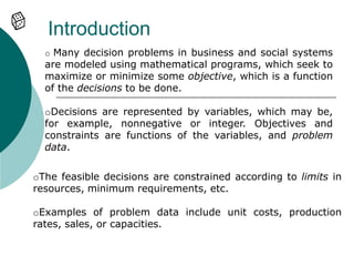
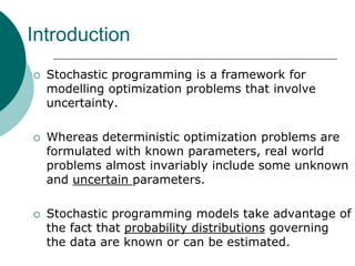
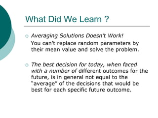
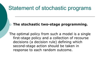
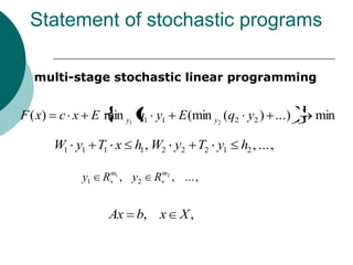
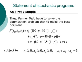
Lecture 1


Introduction. Statement of stochastic
programming problems
Leonidas Sakalauskas
Institute of Mathematics and Informatics
Vilnius, Lithuania <sakal@ktl.mii.lt>

EURO Working Group on Continuous Optimization
Content
   Introduction
   Example
   Basics of Probability
   Unconstrained Stochastic Optimization
   Nonlinear Stochastic Programming
   Two-stage linear Programming
   Multi-Stage Linear Programming
Introduction
  o Many decision problems in business and social systems
  are modeled using mathematical programs, which seek to
  maximize or minimize some objective, which is a function
  of the decisions to be done.

  oDecisions are represented by variables, which may be,
  for example, nonnegative or integer. Objectives and
  constraints are functions of the variables, and problem
  data.

oThe feasible decisions are constrained according to limits in
resources, minimum requirements, etc.

oExamples of problem data include unit costs, production
rates, sales, or capacities.
Introduction
   Stochastic programming is a framework for
    modelling optimization problems that involve
    uncertainty.

   Whereas deterministic optimization problems are
    formulated with known parameters, real world
    problems almost invariably include some unknown
    and uncertain parameters.

   Stochastic programming models take advantage of
    the fact that probability distributions governing
    the data are known or can be estimated.
Introduction
   The goal here is to find some policy that is
    feasible for all (or almost all) the possible data
    change scenarios and maximizes (or minimizes)
    the probability of some event or expectation of
    some function depending on the decisions and
    the random variables.
   This course is aimed to give the knowledge
    about the statement and solving of stochastic
    linear and nonlinear programs
   The issues are also emphasized on continuous
    optimization and applicability of programs
Introduction

Applications
 Sustainability and Power Planning

 Supply Chain Management

 Network optimization

 Logistics

 Financial Management

 Location Analysis

 Activity–Based Costing (ABC)

 Bayesian analysis

 etc.
Introduction

Sources:
   www.stoprog.org

   J. Birge & F. Louvaux (1997) Introduction to
    Stochastic Programming. Springer

   L.Sakalauskas (2006)Towards Implementable
    Nonlinear Stochastic Programming. Lecture
    Notes in Economics and Mathematical
    Systems, vol. 581, pp. 257-279
Introduction
An First Example

   Farmer Fred can plant his land with either
    corn, wheat, or beans.
   For simplicity, assume that the season will
    either be wet or dry – nothing in between.
   If it is wet, corn is the most profitable
   If it is dry, wheat is the most profitable.
Profit

             All Corn   All Wheat    All Beans
     Wet        100          70             80
     Dry         -10         40             35

Assume the probability of a wet season is p,
the expected profit of planting the different crops:
   Corn: -10 + 110p
   Wheat: 40 + 30p
   Beans: 35 + 45p
What is the answer ?

Suppose p = 0.5, can anyone suggest a
  planting plan?

     Plant 1/2 corn, 1/2 wheat ?

Expected Profit:

    0.5 (-10 + 110(0.5)) + 0.5 (40 +
  30(0.5))= 50

Is this optimal?
!!!
Suppose p = 0.5, can anyone suggest a
  planting plan?

Plant all beans!

Expected Profit: 35 + 45(0.5) = 57.5!

The expected profit in behaving optimally is
  15% better than in behaving reasonably !
What Did We Learn ?
   Averaging Solutions Doesn’t Work!
    You can’t replace random parameters by
    their mean value and solve the problem.

   The best decision for today, when faced
    with a number of different outcomes for the
    future, is in general not equal to the
    “average” of the decisions that would be
    best for each specific future outcome.
Statement of stochastic programs
   Mathematical Programming.
The general form of a mathematical program is
 minimize           f(x1, x2,..., xn)     - objective function
 subject to          g1(x1, x2,..., xn) ≤ 0
                                ..           - constraints
                       gm(x1, x2,..., xn) ≤ 0
where the vector
                      x=(x1, x2,..., xn) ϵ X,

supposes the decisions should be done, X is a set that be,
  e.g., all nonnegative real numbers.
For example, xi can represent amount of production of the
  ith from n products.
Statement of stochastic programs
    Stochastic programming


        is like mathematical (deterministic) programming but with
    “random” parameters. Denote E as symbol of expectation and
    Prob as symbol of probability.

Thus, now the objective (or constraint) function becomes by
  mathematical expectation of some random function :

               F(x)=Ef(x, ζ),
or probability of some event A(x):

               F(x)=Prob(ζ ϵ A(x))
x=(x1, x2,..., xn) is a vector of a decision variable, ζ is a vector of
  random variables, defining the uncertainty (scenarios, outcome
  of some experiment).
Statement of stochastic programs

     It makes sense to do just a bit of review of
      probability.

  ζ ϵ Ω is “outcome” of a random experiment,
     called by an elementary event.

      The set of all possible outcomes is Ω.

  The outcomes can be combined into subsets
    A   Ω of ζ (called by events).
Random variable

    Random variable ζ is described by

    1) Set of support Ω=SUPP(ζ)
    2) Probability measure

    Probability measure is defined by the
    cumulative distribution function:

F ( x) Pr ob ( X   x) Pr ob ( X 1   x1 ,..., X n   xn )
Probabilistic measure
 Probabilistic
             measure can have
 only three components:
             Continuous;
             Discrete (integer);
             Singular.
Continuous r.v.


Continuous random variable (or random
 vector) are defined by probability density
 function:
                          n
              p( z ) :
   Thus, in an uni-variate case:
                   x
          F ( x)       p( z )dz
Continuous r.v.


If the probability measure is absolutely
   continuous, the expected value of
   random function f (x, ) is integral:


 F ( x)   Ef ( x, )   f ( x, z ) p( z )dz
Continuous r.v.

  The probability of some event (set of scenarios)
   A is defined by the integral, too:

        Pr ob (      A)        Eh( )     p ( z )dz
                                       z A

where
                      1,          A
              h( )
                          0,      A
is the characteristic-function of set A.
What did we learn ?

 Remark. Since any nonnegative function
                    n
               p:
 that
              p ( z )dz 1

is the density function of certain random
variable (or vector) some multivariate
integrals can be changed by expectation of
some random variable (or vector).
Discrete r. v.
Discrete r.v. ζ is described by mass
  probabilities of all elementary events:

            z1 , z 2 ,..., z K
            p1 , p2 ,..., pK ,
that


       p1     p2 ... pK          1
Discrete r. v.
If probability measure is discrete, the expected
value of random function is the sum or series:


                   K
        Ef ( X )         f ( zi ) pi
                   i 1
Singular random variable


Singular r.v. probabilistic measure is
  concentrated on the set having the
  zero Borel measure (say, the Cantor
  set).
Statement of stochastic programs

   Unconstrained continuous (nonlinear)
    stochastic programming problem:

       F ( x)   Ef x,   f ( x, z ) p( z )dz   min
       x   X.

It is easy to extend this statement to discrete
model of uncertainty and constrained
optimization
Statement of stochastic programs

   Constrained continuous (nonlinear )stochastic
    programming problem is

     F0 ( x)   Ef 0 x,           n
                                     f 0 ( x, z ) p( z )dz     min
                             R

     F1 ( x)   Ef1 x,            n
                                     f1 ( x, z ) p( z )dz 0,
                             R

                         x           X.
If the constraint function is the probability of some
event depending on the decision variable, the problem
becomes by chance-constrained stochastic
programming problem
Statement of stochastic programs

    Note, the expectation can enter the objective
    function by nonlinear way, i.e.


             F ( x)    Ef x,      min
             x X.

Programs with functions of such kind are often
considered in statistics: Bayesian analysis, likelihood
estimation, etc., that are solved by Monte-Carlo
Markov Chain (MCMC) approach.
Statement of stochastic programs

   The stochastic two-stage programming.

The most widely applied and studied stochastic
  programming models are two-stage linear programs.

Here the decision maker takes some action in the first
  stage, after which a random event occurs affecting the
  outcome of the first-stage decision.

A recourse decision can then be made in the second
   stage that compensates for any bad or undesired effects
   that might have been experienced as a result of the
   first-stage decision.
Statement of stochastic programs

   The stochastic two-stage programming.

The optimal policy from such a model is a single
  first-stage policy and a collection of recourse
  decisions (a decision rule) defining which
  second-stage action should be taken in
  response to each random outcome.
Statement of stochastic programs

 two-stage stochastic linear programming

  The two-stage stochastic linear programming (SLP) problem
  with recourse is formulated as


     F ( x) c x E min y q y                min

         W y T x h,             y   Rm ,

                 Ax b, x         X,
assume vectors q, h and matrices W, T be random in general.
Statement of stochastic programs

  multi-stage stochastic linear programming


F ( x) c x E min y1 q1 y1 E (min y2 (q2 y2 ) ...)       min

      W1 y1 T1 x h1, W2 y2 T2 y1           h2 , ... ,

           y1   R m1 , y2   R m2 , ... ,


                 Ax b, x           X,
Statement of stochastic programs
    An First Example

    Thus, Farmer Tedd have to solve the
    optimization problem that to make the best
    decision:

   F ( x1 , x2 , x3 ) x1 (100 p 10 (1 p))
                    x2 (70 p 40 (1 p))
                    x3 (80 p 35 (1 p))        max

subject to    x1    0, x2   0, x3   0,      x1 x2   x3 1.
Wrap-up and conclusions
   Stochastic programming problems are
    formulated as mathematical programming
    tasks with the objective and constraints
    defined as expectations of some random
    functions or probabilities of some sets of
    scenarios
   Expectations are defined by multivariate
    integrals (scenarios distributed
    continuously) or finite series (scenarios
    distributed discretely).

Statement of stochastic programming problems

  • 1.
    Lecture 1 Introduction. Statementof stochastic programming problems Leonidas Sakalauskas Institute of Mathematics and Informatics Vilnius, Lithuania <sakal@ktl.mii.lt> EURO Working Group on Continuous Optimization
  • 2.
    Content  Introduction  Example  Basics of Probability  Unconstrained Stochastic Optimization  Nonlinear Stochastic Programming  Two-stage linear Programming  Multi-Stage Linear Programming
  • 3.
    Introduction oMany decision problems in business and social systems are modeled using mathematical programs, which seek to maximize or minimize some objective, which is a function of the decisions to be done. oDecisions are represented by variables, which may be, for example, nonnegative or integer. Objectives and constraints are functions of the variables, and problem data. oThe feasible decisions are constrained according to limits in resources, minimum requirements, etc. oExamples of problem data include unit costs, production rates, sales, or capacities.
  • 4.
    Introduction  Stochastic programming is a framework for modelling optimization problems that involve uncertainty.  Whereas deterministic optimization problems are formulated with known parameters, real world problems almost invariably include some unknown and uncertain parameters.  Stochastic programming models take advantage of the fact that probability distributions governing the data are known or can be estimated.
  • 5.
    Introduction  The goal here is to find some policy that is feasible for all (or almost all) the possible data change scenarios and maximizes (or minimizes) the probability of some event or expectation of some function depending on the decisions and the random variables.  This course is aimed to give the knowledge about the statement and solving of stochastic linear and nonlinear programs  The issues are also emphasized on continuous optimization and applicability of programs
  • 6.
    Introduction Applications  Sustainability andPower Planning  Supply Chain Management  Network optimization  Logistics  Financial Management  Location Analysis  Activity–Based Costing (ABC)  Bayesian analysis  etc.
  • 7.
    Introduction Sources:  www.stoprog.org  J. Birge & F. Louvaux (1997) Introduction to Stochastic Programming. Springer  L.Sakalauskas (2006)Towards Implementable Nonlinear Stochastic Programming. Lecture Notes in Economics and Mathematical Systems, vol. 581, pp. 257-279
  • 8.
    Introduction An First Example  Farmer Fred can plant his land with either corn, wheat, or beans.  For simplicity, assume that the season will either be wet or dry – nothing in between.  If it is wet, corn is the most profitable  If it is dry, wheat is the most profitable.
  • 9.
    Profit All Corn All Wheat All Beans Wet 100 70 80 Dry -10 40 35 Assume the probability of a wet season is p, the expected profit of planting the different crops: Corn: -10 + 110p Wheat: 40 + 30p Beans: 35 + 45p
  • 10.
    What is theanswer ? Suppose p = 0.5, can anyone suggest a planting plan? Plant 1/2 corn, 1/2 wheat ? Expected Profit: 0.5 (-10 + 110(0.5)) + 0.5 (40 + 30(0.5))= 50 Is this optimal?
  • 11.
    !!! Suppose p =0.5, can anyone suggest a planting plan? Plant all beans! Expected Profit: 35 + 45(0.5) = 57.5! The expected profit in behaving optimally is 15% better than in behaving reasonably !
  • 12.
    What Did WeLearn ?  Averaging Solutions Doesn’t Work! You can’t replace random parameters by their mean value and solve the problem.  The best decision for today, when faced with a number of different outcomes for the future, is in general not equal to the “average” of the decisions that would be best for each specific future outcome.
  • 13.
    Statement of stochasticprograms  Mathematical Programming. The general form of a mathematical program is minimize f(x1, x2,..., xn) - objective function subject to g1(x1, x2,..., xn) ≤ 0 .. - constraints gm(x1, x2,..., xn) ≤ 0 where the vector x=(x1, x2,..., xn) ϵ X, supposes the decisions should be done, X is a set that be, e.g., all nonnegative real numbers. For example, xi can represent amount of production of the ith from n products.
  • 14.
    Statement of stochasticprograms Stochastic programming   is like mathematical (deterministic) programming but with “random” parameters. Denote E as symbol of expectation and Prob as symbol of probability. Thus, now the objective (or constraint) function becomes by mathematical expectation of some random function : F(x)=Ef(x, ζ), or probability of some event A(x): F(x)=Prob(ζ ϵ A(x)) x=(x1, x2,..., xn) is a vector of a decision variable, ζ is a vector of random variables, defining the uncertainty (scenarios, outcome of some experiment).
  • 15.
    Statement of stochasticprograms  It makes sense to do just a bit of review of probability. ζ ϵ Ω is “outcome” of a random experiment, called by an elementary event. The set of all possible outcomes is Ω. The outcomes can be combined into subsets A Ω of ζ (called by events).
  • 16.
    Random variable Random variable ζ is described by 1) Set of support Ω=SUPP(ζ) 2) Probability measure Probability measure is defined by the cumulative distribution function: F ( x) Pr ob ( X x) Pr ob ( X 1 x1 ,..., X n xn )
  • 17.
    Probabilistic measure  Probabilistic measure can have only three components:  Continuous;  Discrete (integer);  Singular.
  • 18.
    Continuous r.v. Continuous randomvariable (or random vector) are defined by probability density function: n p( z ) : Thus, in an uni-variate case: x F ( x) p( z )dz
  • 19.
    Continuous r.v. If theprobability measure is absolutely continuous, the expected value of random function f (x, ) is integral: F ( x) Ef ( x, ) f ( x, z ) p( z )dz
  • 20.
    Continuous r.v. The probability of some event (set of scenarios) A is defined by the integral, too: Pr ob ( A) Eh( ) p ( z )dz z A where 1, A h( ) 0, A is the characteristic-function of set A.
  • 21.
    What did welearn ? Remark. Since any nonnegative function n p: that p ( z )dz 1 is the density function of certain random variable (or vector) some multivariate integrals can be changed by expectation of some random variable (or vector).
  • 22.
    Discrete r. v. Discreter.v. ζ is described by mass probabilities of all elementary events: z1 , z 2 ,..., z K p1 , p2 ,..., pK , that p1 p2 ... pK 1
  • 23.
    Discrete r. v. Ifprobability measure is discrete, the expected value of random function is the sum or series: K Ef ( X ) f ( zi ) pi i 1
  • 24.
    Singular random variable Singularr.v. probabilistic measure is concentrated on the set having the zero Borel measure (say, the Cantor set).
  • 25.
    Statement of stochasticprograms  Unconstrained continuous (nonlinear) stochastic programming problem: F ( x) Ef x, f ( x, z ) p( z )dz min x X. It is easy to extend this statement to discrete model of uncertainty and constrained optimization
  • 26.
    Statement of stochasticprograms  Constrained continuous (nonlinear )stochastic programming problem is F0 ( x) Ef 0 x, n f 0 ( x, z ) p( z )dz min R F1 ( x) Ef1 x, n f1 ( x, z ) p( z )dz 0, R x X. If the constraint function is the probability of some event depending on the decision variable, the problem becomes by chance-constrained stochastic programming problem
  • 27.
    Statement of stochasticprograms Note, the expectation can enter the objective function by nonlinear way, i.e. F ( x) Ef x, min x X. Programs with functions of such kind are often considered in statistics: Bayesian analysis, likelihood estimation, etc., that are solved by Monte-Carlo Markov Chain (MCMC) approach.
  • 28.
    Statement of stochasticprograms  The stochastic two-stage programming. The most widely applied and studied stochastic programming models are two-stage linear programs. Here the decision maker takes some action in the first stage, after which a random event occurs affecting the outcome of the first-stage decision. A recourse decision can then be made in the second stage that compensates for any bad or undesired effects that might have been experienced as a result of the first-stage decision.
  • 29.
    Statement of stochasticprograms  The stochastic two-stage programming. The optimal policy from such a model is a single first-stage policy and a collection of recourse decisions (a decision rule) defining which second-stage action should be taken in response to each random outcome.
  • 30.
    Statement of stochasticprograms two-stage stochastic linear programming The two-stage stochastic linear programming (SLP) problem with recourse is formulated as F ( x) c x E min y q y min W y T x h, y Rm , Ax b, x X, assume vectors q, h and matrices W, T be random in general.
  • 31.
    Statement of stochasticprograms multi-stage stochastic linear programming F ( x) c x E min y1 q1 y1 E (min y2 (q2 y2 ) ...) min W1 y1 T1 x h1, W2 y2 T2 y1 h2 , ... , y1 R m1 , y2 R m2 , ... , Ax b, x X,
  • 32.
    Statement of stochasticprograms An First Example Thus, Farmer Tedd have to solve the optimization problem that to make the best decision: F ( x1 , x2 , x3 ) x1 (100 p 10 (1 p)) x2 (70 p 40 (1 p)) x3 (80 p 35 (1 p)) max subject to x1 0, x2 0, x3 0, x1 x2 x3 1.
  • 33.
    Wrap-up and conclusions  Stochastic programming problems are formulated as mathematical programming tasks with the objective and constraints defined as expectations of some random functions or probabilities of some sets of scenarios  Expectations are defined by multivariate integrals (scenarios distributed continuously) or finite series (scenarios distributed discretely).