Download as PDF, PPTX

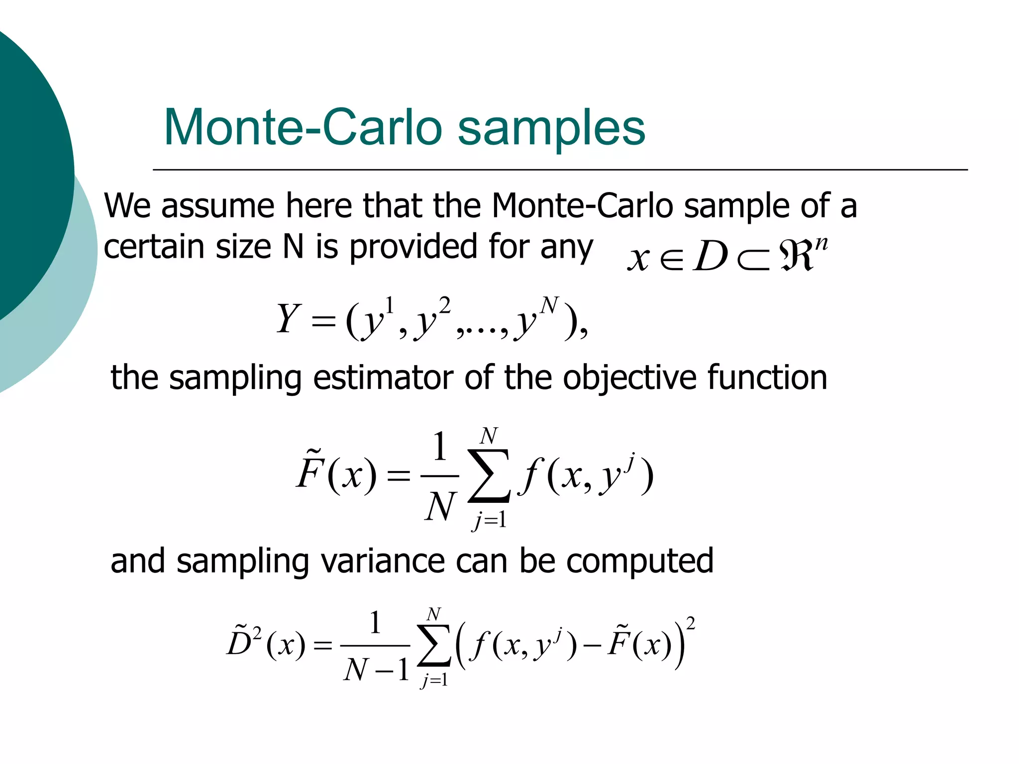
![Two-stage stochastic optimization
problem
F ( x) c x E min y [q y | W y T x h, y R ] min
m
Ax b, x n ,
assume vectors q, h and matrices W, T random in
general.](https://image.slidesharecdn.com/lecture5-100818114346-phpapp01/75/Monte-Carlo-method-for-Two-Stage-SLP-3-2048.jpg)
![Two-stage stochastic optimization problem with
complete recourse will be
F ( x ) c x E Q ( x, ) min n
xD
subject to the feasible set
D x A x b, x R
n
where
Q( x, ) min y [q y | W y T x h, y R ]
m](https://image.slidesharecdn.com/lecture5-100818114346-phpapp01/75/Monte-Carlo-method-for-Two-Stage-SLP-6-2048.jpg)
![It can be derived under the assumption on the existence
of a solution at the second stage and continuity of
measure P, that the objective function is smoothly
differentiable and the gradient is
x F ( x) Eg ( x, )
where
g ( x, ) c T u *
is given by the set of solutions of the dual problem
(h T x)T u * max u [(h T x)T u | u W T q 0, u R ]
s](https://image.slidesharecdn.com/lecture5-100818114346-phpapp01/75/Monte-Carlo-method-for-Two-Stage-SLP-7-2048.jpg)
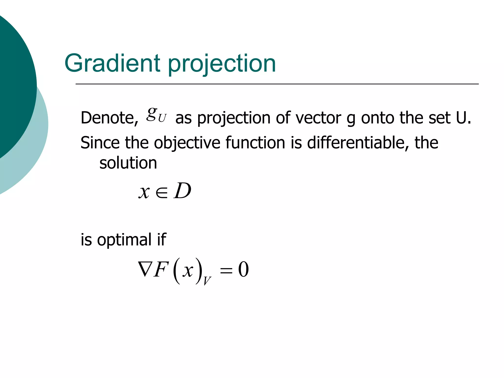
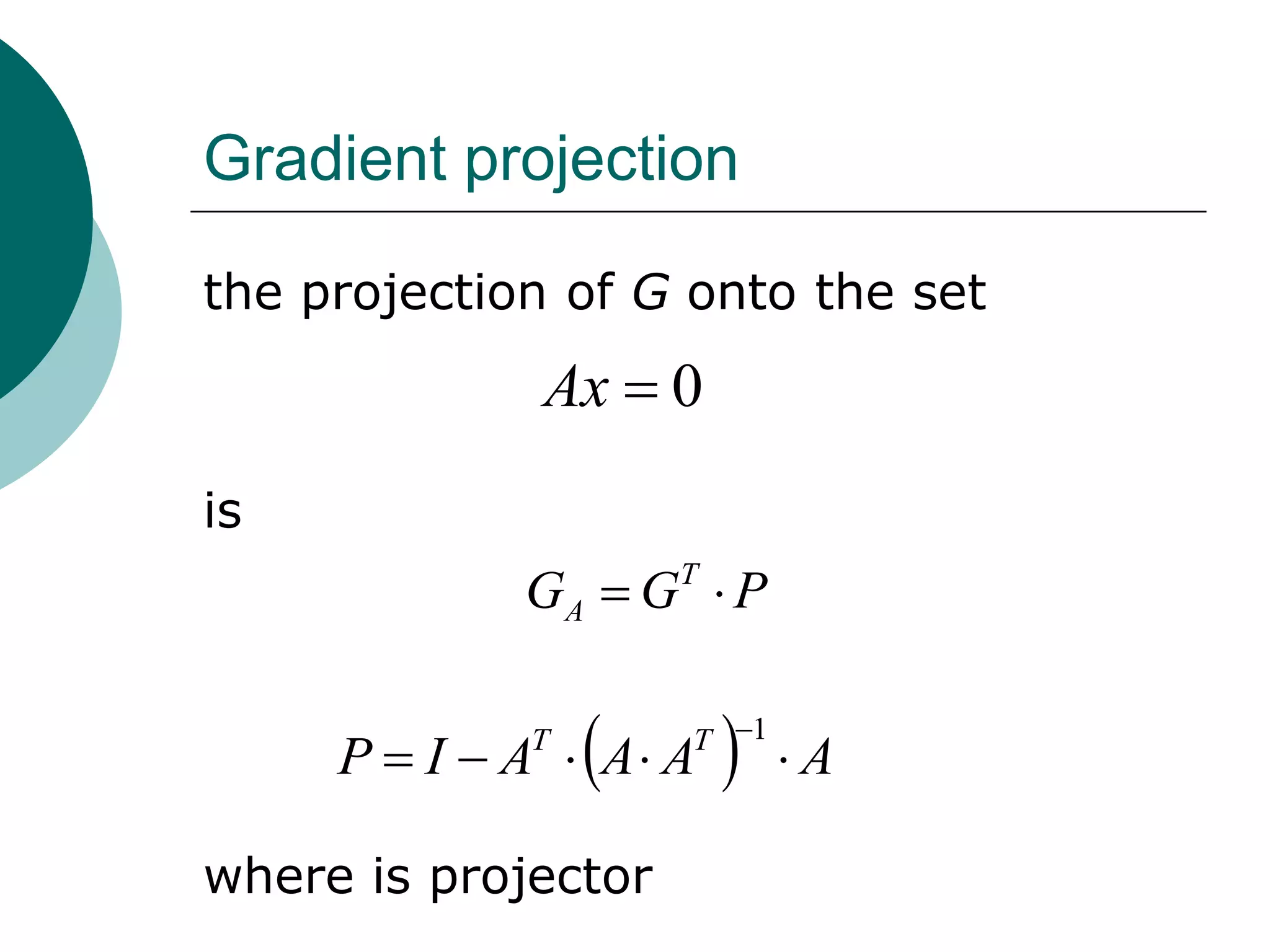
![The starting point can be obtained as the solution of the
deterministic linear problem:
( x 0 , y 0 ) arg min[c x q y | A x b, W y T x h, y R , x R ].
m n
x, y
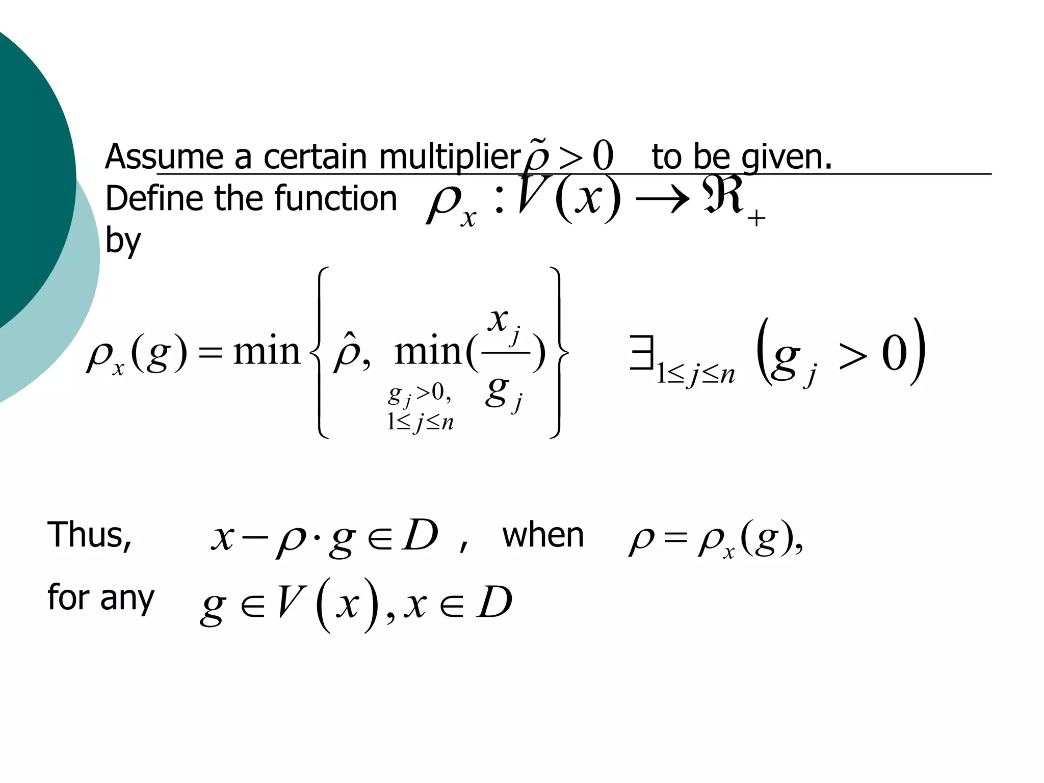
The iterative stochastic procedure of gradient search could
be used further:
xt 1 xt t G ( xt )
where t t (Gt ) is the step-length multiplier and
x
G G( xt )
t
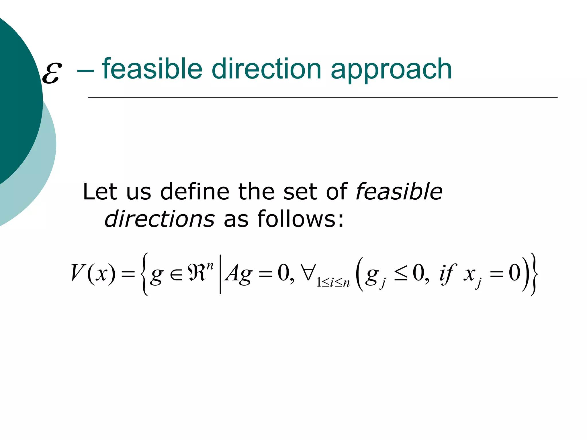
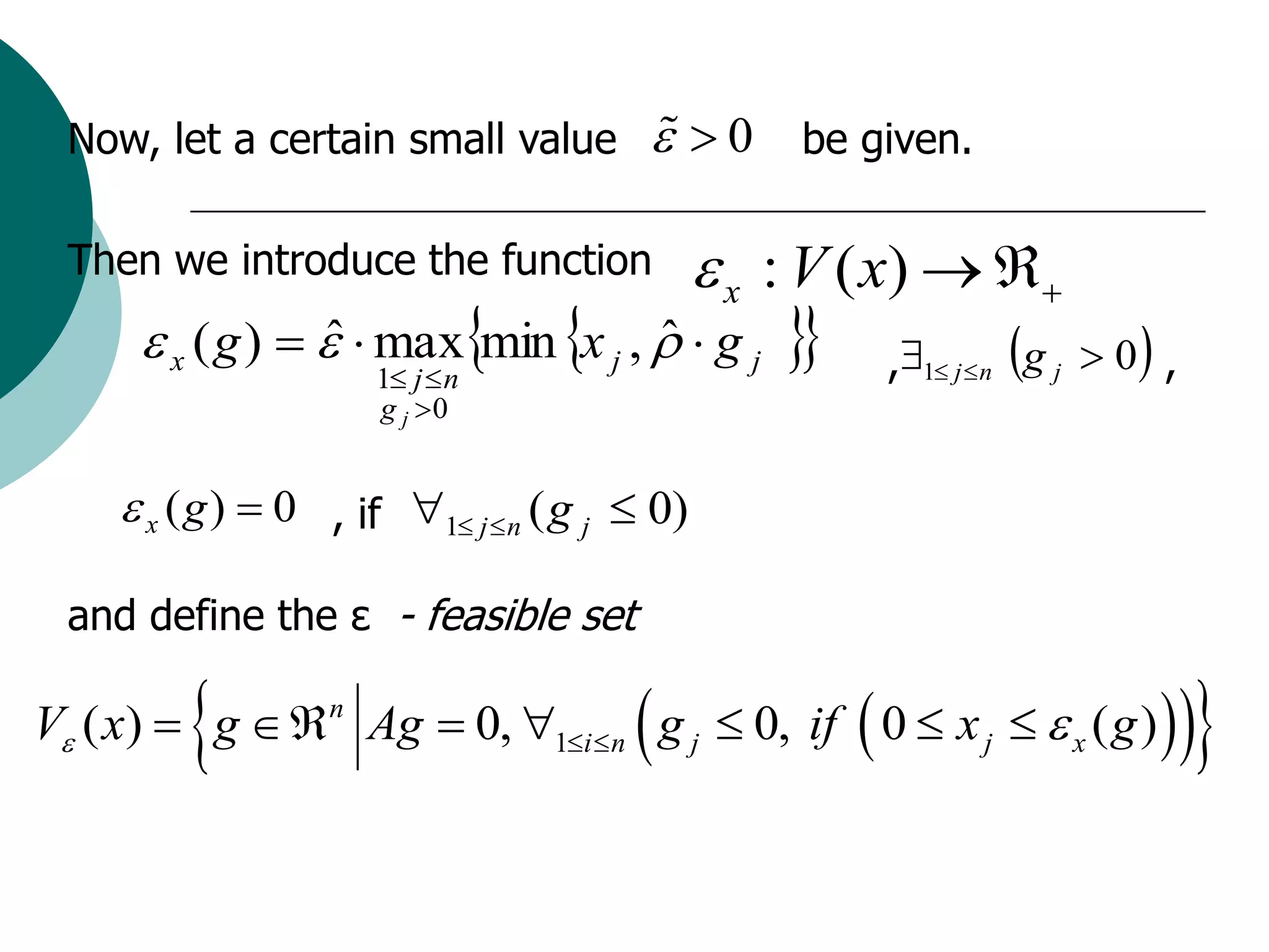
-feasible the projection of gradient
estimator to the ε
is set.
V xt](https://image.slidesharecdn.com/lecture5-100818114346-phpapp01/75/Monte-Carlo-method-for-Two-Stage-SLP-16-2048.jpg)
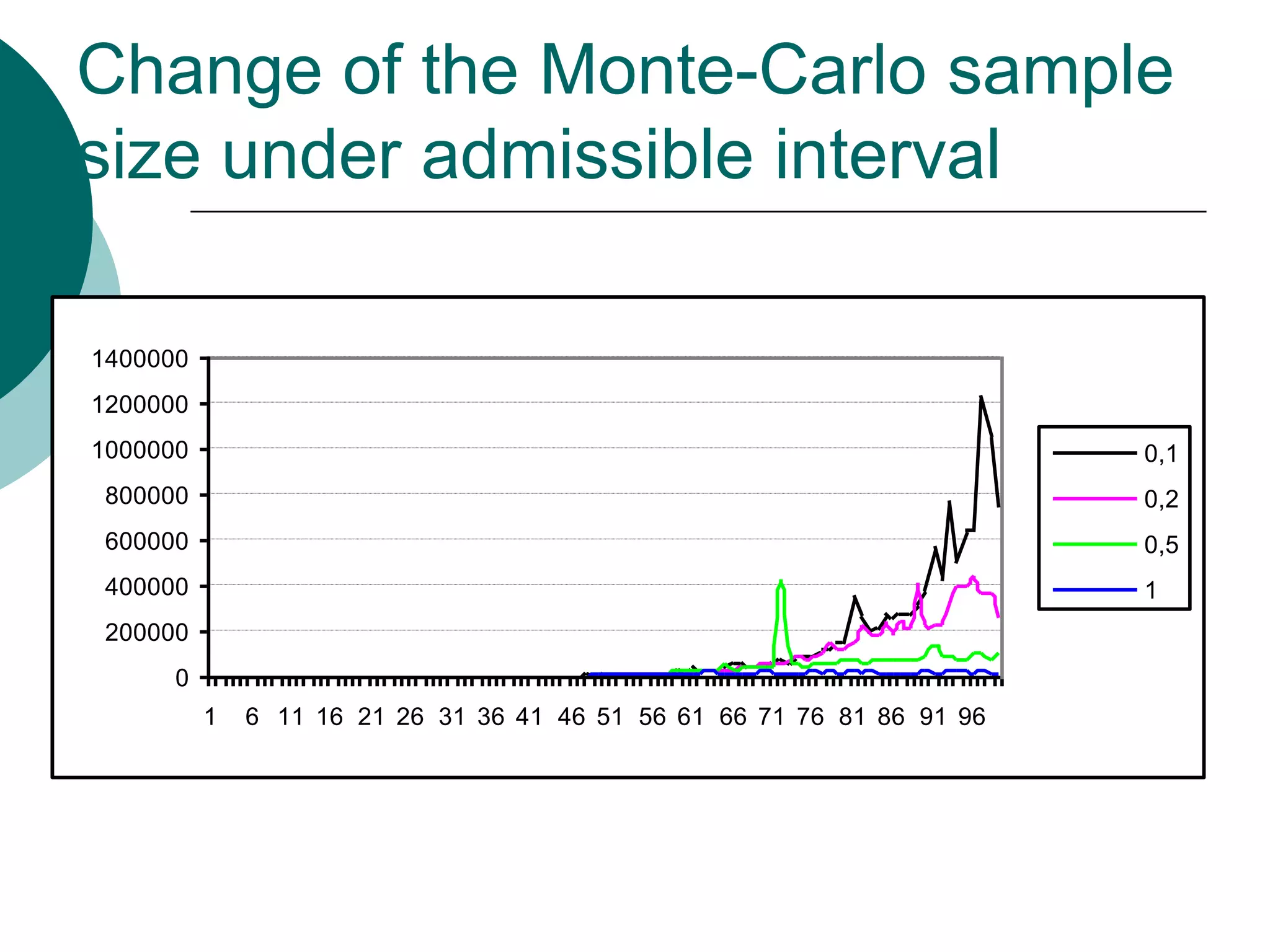
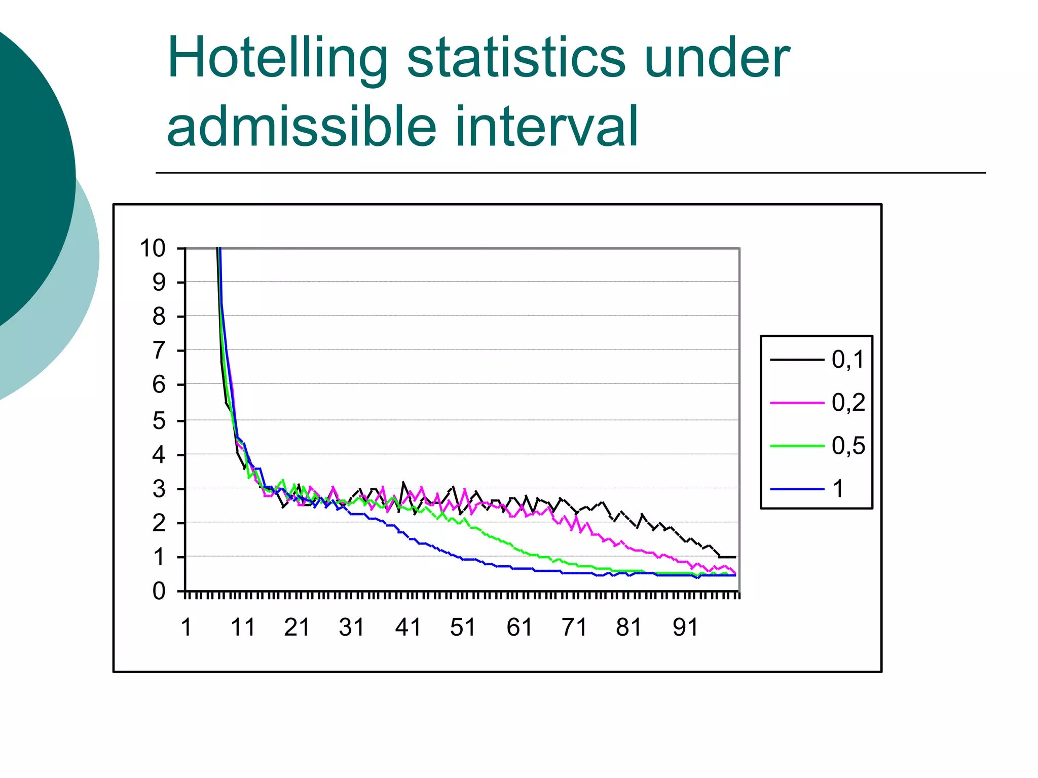
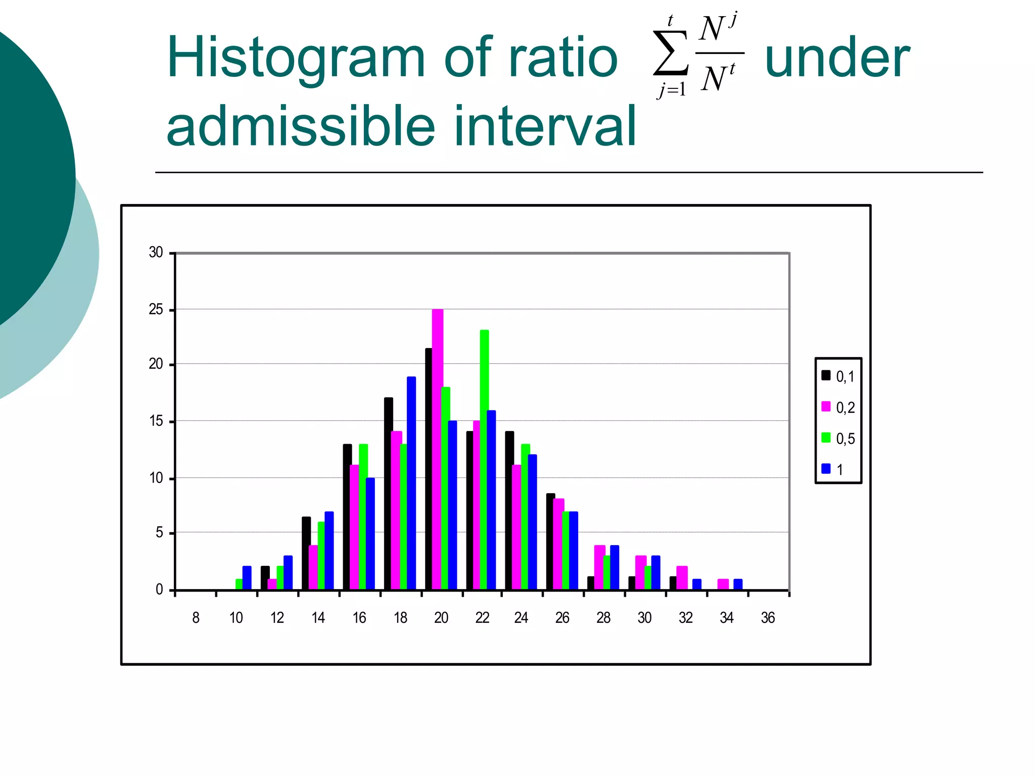

This document presents a detailed lecture on the Monte Carlo method for solving two-stage stochastic linear programming problems, focusing on various estimation techniques and optimality testing. It outlines the iterative stochastic procedure for gradient search and discusses methods for regulating sample sizes during optimization. The conclusions emphasize the development of a stochastic adaptive method that ensures convergence through adjustments based on Monte Carlo estimates and statistical accuracy.